An Overview of Information Flow in AMBER
Overview
Teaching: 30 min
Exercises: 5 minQuestions
What files are needed to run an MD simulation with AMBER?
Objectives
Learn what types of files are needed to run an MD simulation with AMBER
Introduction
Information flow in AMBER
Simulation workflow in MD usually involves three steps: system preparation, simulation, and analysis. Let’s take a closer look at these steps.
coordinates| C{TLEAP,
XLEAP} B([FF files]) --> |Load
parameters|C H([LEaP commands])-->|Build
simulation system|C end subgraph "Run MD" C-->|Save
topology|D(["prmtop"]) C==>|Save
coordinates|E(["inpcrd"]) E==>|Load
coordinates|F Q([disang])-.->|Load
NMR restraints|F T([groupfile])-.->|Setup
multiple
simulations|F G(["mdin"])-->|Load
run options|F D-->|Load
topology|F{SANDER,
PMEMD} F==>|Save
restart|P([restrt]) P==>|Load
restart|F end subgraph Analyze N(["CPPTRAJ
commands"])-->|Run
analysis|J F===>|Save
trajectory|I([mdcrd, mdvel]) F--->|Print
energies|L([mdout,
mdinfo]) L-->|Load
energies|J I==>|Load
frames|J{CPPTRAJ,
PYTRAJ} I==>|Load
frames|K{MMPBSA} R([MM-PBSA
commands])-.->|Compute
PB energy|K J-->S[Results] K--->S((Results)) end D---->|Load
topology|J linkStyle 1,3,9,21 fill:none,stroke:blue,stroke-width:3px; linkStyle 2,8,12 fill:none,stroke:red,stroke-width:3px;
System Preparation
- Two utilities for simulation preparation: tLEaP and xLEaP.
- The command line version (tLeap) is very efficient for executing scripts automatically.
- The GUI version (xLEaP) is good for building simulation systems interactively.
Simulation
- Two MD engines: SANDER and PMEMD.
- Parallel (MPI) SANDER
- Parallel and GPU-accelerated PMEMD
- PMEMD is faster than SANDER, but it has fewer options
Analysis
- CPPTRAJ (command-line pytraj)
- PYTRAJ (python front end to ptraj)
- MMPBSA
Other useful utilities:
- antechamber (topology builder)
- parmed (utility for topology editing and conversion)
- quick (GPU-accelerated DFT QM program)
- packmol-memgen (utility for preparing membrane systems)
Key Points
To run an MD simulation with AMBER 3 files are needed: an input file, a parameter file, and a file describing coordinates/velocities .
Checking and Preparing PDB Files
Overview
Teaching: 20 min
Exercises: 10 minQuestions
What problems are commonly found in PDB files?
Why fixing errors in PDB files is essential for a simulation?
Objectives
Understand why it is necessary to check PDB files before simulation.
Learn how to look for problems in PDB files.
Learn how to fix the common errors in PDB files.
What data is needed to setup a simulation?
- Molecular simulation systems are typically prepared from PDB files.
- For a simulation to be setup, only the coordinate section consisting of ATOM, HETATM, and TER records is required.
         atomName  chain            coordinates                temperatureFactor (beta)
             |       |            x       y       z             |
ATOM      1  N   MET A   1      39.754  15.227  24.484  1.00 46.61
                 |       |                               |
           residueName  residueID                       occupancy

ATOM    147  CG AASP A  20      53.919   7.536  24.768  0.50 31.95
ATOM    148  CG BASP A  20      55.391   5.808  23.334  0.50 32.16
                |
               conformation

TER  - indicates the end of a chain

HETATM  832  O   HOH A 106      32.125   6.262  24.443  1.00 21.18
- The lines beginning with “ATOM” represent the atomic coordinates for standard amino acids and nucleotides.
- For chemical compounds other than proteins or nucleic acids, the “HETATM” record type is used.
- Records of both types use a simple fixed-column format explained here.
- “TER” records indicate which atoms are at the end of a protein chain.
Important Things to Check in a PDB File
A correct simulation of molecules requires error-free input PDB files.
There are several common problems with PDB files, including:
- presence of non-protein molecules (crystallographic waters, ligands, modified amino acids, etc.)
- alternate conformations
- missing side-chain atoms
- missing fragments
- clashes between atoms
- multiple copies of the same protein chains
- di-sulfide bonds
- wrong assignment of the N and O atoms in the amide groups of ASN and GLN, and the N and C atoms in the imidazole ring of HIS
Connect to the training cluster
Sign in to the training cluster jupyter.md-workshop.ace-net.training. Start a server with the following arguments:
- 4 CPUs
- 4 hours
- default RAM
- 1 GPUs
Workshop data:
On the training cluster copy archive in your home directory and unpack:
cd
cp /project/def-sponsor00/workshop_amber_2024.tar.gz .
tar xf workshop_amber_2024.tar.gz
Checking a molecular structure
- Check_structure is a command-line utility from BioBB project for exhaustive structure quality checking.
Installing check_structure.
module load StdEnv/2023 python scipy-stack
virtualenv ~/env-biobb
source ~/env-biobb/bin/activate
pip install biobb-structure-checking
Using check_structure.
cd ~/workshop_amber/example_01
check_structure commands # print help on commands
check_structure -i 2qwo.pdb checkall
...
Detected no residues with alternative location labels
...
Found 154 Residues requiring selection on adding H atoms
...
Detected 348 Water molecules
...
Detected 8 Ligands
...
Detected 1 Possible SS Bonds
...
No severe clashes detected
Removing Non-Protein Molecules
Let’s remove ligands and save the output in a new file called “protein.pdb”.
check_structure -i 2qwo.pdb -o protein.pdb ligands --remove all
Selecting protein atoms using VMD
Select only protein atoms from the file
2qwo.pdband save them in the new fileprotein.pdbusing VMD.Solution
Load vmd module and start the program:
module load StdEnv/2023 vmd
vmd
mol new 2qwo.pdb set prot [atomselect top "protein"] $prot writepdb protein.pdb quitThe first line of code loads a new molecule from 2qwo.pdb. Using the atomselect method, we then select all protein atoms from the top molecule. Finally, we save the selection in the file “protein.pdb”.
The Atom Selection Language has many capabilities. You can learn more about it by visiting the following webpage.
Selecting protein atoms using shell commands
Standard Linux text searching utility
grepcan find and print all “ATOM” records from a PDB file. This is a good example of using Unix command line, andgrepis very useful for many other purposes such as finding important things in log files.Grepsearches for a given pattern in files and prints out each line that matches a pattern.
- Check if a PDB file has “HETATM” records using
grepcommand.- Select only protein atoms from the file
2qwo.pdband save them in the new fileprotein.pdbusinggrepcommand to select protein atoms (the “ATOM” and the “TER” records).Hint: the
ORoperator in grep is\|. The output from a command can be redirected into a file using the output redirection operator>.Solution
1.
grep "^HETATM " 1ERT.pdb | wc -l46The
^expression matches beginning of line. We used thegrepcommand to find all lines beginning with the word “HETATM” and then we sent these lines to the character counting commandwc. The output tells us that the downloaded PDB file contains 46 non-protein atoms. In this case, they are just oxygen atoms of the crystal water molecules.2.
grep "^ATOM\|^TER " 1ERT.pdb > protein.pdb
Checking PDB Files for alternate conformations.
Check conformations
cd ~/workshop_amber/example_02
check_structure -i 1ert.pdb checkall
ASP A20
  CG   A (0.50) B (0.50)
  OD1  A (0.50) B (0.50)
  OD2  A (0.50) B (0.50)
HIS A43
  CG   A (0.50) B (0.50)
  ND1  A (0.50) B (0.50)
  CD2  A (0.50) B (0.50)
  CE1  A (0.50) B (0.50)
  NE2  A (0.50) B (0.50)
SER A90
  OG   A (0.50) B (0.50)
Select conformers A ASP20 and B HIS43.
check_structure -i 1ert.pdb -o output.pdb altloc --select A20:A,A43:B,A90:B
Selecting Alternate Conformations with VMD
- Check if the file 1ERT.pdb has any alternate conformations.
- Select conformation A for residues 43, 90. Select conformation B for residue 20. Save the selection in the file “protein_20B_43A_90A.pdb”.
Solution
1.
mol new 1ert.pdb
set s [atomselect top "altloc A"]
$s get resid
set s [atomselect top "altloc B"]
$s get resid
$s get {resid resname name}
set s [atomselect top "altloc C"]
$s get resid
quit
The output of the commands tells us that residues 20, 43 and 90 have alternate conformations A and B.
2.
mol new 1ERT.pdb
set s [atomselect top "(protein and altloc '') or (altloc B and resid 20) or (altloc A and resid 43 90)"]
$s writepdb protein_20B_43A_90A.pdb
quit
Checking PDB Files for cross-linked cysteines.
- For simulation preparation with the AMBER, cross-linked cysteines must be renamed from “CYS” to “CYX”
cd ~/workshop_amber/example_01
check_structure -i 2qwo.pdb -o output.pdb getss --mark all
grep CYX output.pdb
- GROMACS
pdb2gmxutility can automatically add S-S bonds to the topology based on the distance between sulfur atoms (option -ss).
Useful Links
MDWeb server can help to identify problems with PDB files and visually inspect them. It can also perform complete simulation setup, but options are limited and waiting time in the queue may be quite long.
CHARMM-GUI can be used to generate input files for simulation with CHARMM force fields. CHARMM-GUI offers useful features, for example the “Membrane Builder” and the “Multicomponent Assembler”.
Key Points
Small errors in the input structure may cause MD simulations to became unstable or give unrealistic results.
Assigning Protonation States to Residues in a Protein
Overview
Teaching: 30 min
Exercises: 10 minQuestions
Why titratable aminoacid residues can have different protonation states?
How to determine protonation state of a residue in a protein?
What are the weaknesses of fixed protonation state simulations?
Objectives
Understand why it is necessary to assign the correct protonation state
Learn how to determine protonation state of a protein
Learn how to assign protonation state to a residue
It is important to consider amino acid protonation states
- The protonation pattern of proteins is crucial for their catalytic function and structural stability.
- Numerous MD simulation studies have demonstrated the importance of protein protonation states [1, 2, 3, 4, 5].
How to Determine Protonation States of Residues in a Protein?
For predicting the pKa values of protein residues, several web servers and standalone programs are available.
- H++. Continuum electrostatics model
- PROPKA3.0. Empirical pKa prediction.
- PlayMolecule-ProteinPrepare. Based on PROPKA3.
- PDB2PQR. Solves Poisson-Boltzmann equation.
- MCCE. Takes into account conformational flexibility. More accurate and more challenging to use.
- PKAD. A database of experimentally determined pKa values.
There is no perfect pKa prediction method. Deviations from experimental values can sometimes be significant. The best practice is to compare the results obtained from different techniques and, if possible, to use experimentally measured values.
Calculating pKa’s
- Calculate pKa’s of residues in the PDB entry 1RGG using H++ server.
- What protonation states of Asp79 and His53 are appropriate for simulation at pH 6?
- Repeat calculations using PDB2PQR server and compare the results.
- Compare calculated pKa’s with the experimental. How accurate are the predicted pKa values?
What protonation states are appropriate for simulating Asp79 and His53 at pH 6?
Solution
If pKa > pH the probability that the residue is protonated is > 50%, and we use the protonated form.
If pKa < pH the probability that the residue is protonated is < 50% and we use the deprotonated form.ASP79 has pKa 7.2 (experimental 7.37), it is protonated at pH 6 and we rename it to ASH
HIS53 has pKa 8.3 (experimental 8.27), it is also protonated at pH 6 and we rename it to HIP
How to select protonation state of a residue?
Assigning protonation states in structure files
- To change the form of an amino acid, change its name in the structure file
LYS (+1) - LYN  (0)
ASP (-1) - ASH  (0)
GLU (-1) - GLH  (0)
HIS  (0) - HIE  (0)
HIS  (0) - HID  (0)
HIS  (0) - HIP (+1)
Selecting protonation states with check_structure.
Let’s change ASP20 and ASP26 in the file 1ert.pdb to the neutral form ASH.
cd ~/workshop_amber/example_02
check_structure -i 1ert.pdb -o 1ert_protonated.pdb \
command_list --list \
"add_hydrogen --add_mode list --list A:asp20ash,A:asp26ash; \
water --remove yes"
You can verify that residues are changed by grepping ASH.
Selecting protonation states with VMD.
Change ASP20 and ASP26 in the file 1ert.pdb to the neutral form ASH and remove water.
Solution
ml StdEnv/2023 vmd
vmd
mol new 1ert.pdb set s [atomselect top "resid 20 26"] $s set resname ASH set s [atomselect top "protein"] $s writepdb 1ert_protonated.pdb quit
Assigning protonation states with the GROMACS pdb2gmx module
- By default, pdb2gmx will select charged forms of LYS, ASP, or GLU
- For HIS, it will try to place the proton optimally
Downsides:
- Interactive
- Residue names are changed only in the topology
Limitations of Fixed Protonation State Simulations
- Difficult to understand proton-coupled conformational dynamics.
- Consider using constant pH simulations if proton-coupled dynamics are essential to your research.
Combining all structure preparation steps in one check_structure script
cd ~/workshop_amber/example_03
check_structure -i 1rgg.pdb -o 1RGG_chain_A_prot.pdb \
    command_list --list "\
        chains --select A;\
        add_hydrogen --list A:his53hip,A:asp79ash --add_mode list;\
        altloc --select A5:B,A54:B,A6:A,A13:A,A42:A,A85:A,A91:A;\
        getss --mark all;\
        ligands --remove all;\
        water --remove yes"
You can also save commands in a file and pass it as an argument to “command_list –list”:
check_structure -i 1rgg.pdb -o 1RGG_chain_A_prot.pdb command_list --list prep_1rgg.chk
References
Combining all structure preparation steps in one VMD script
Combine all previous steps together and create VMD script to prepare MD simulation system for the hydrolaze PDB structure 1RGG. The script should perform the following steps:
- Select molecule A
- Remove non-protein molecules
- Select location ‘B’ for residues 5, 54 and location ‘A’ for all other residues with alternative locations
- Protonate Asp79 and His53
- Rename CYS 7 and 96 into CYX (cross-linked cystein)
- Save the resulting structure as 1RGG_chain_A_prot.pdb
Solution
cd ~/workshop_amber/example_03Save the following commands in a file, e.g. prep_1RGG.vmd
# Load 1rgg.pdb into a new (top) molecule
mol pdbload 1rgg
# Select and save all chain A protein atoms
set s [atomselect top "protein and chain A"]
$s writepdb 1RGG_chain_A.pdb
# Delete the top molecule
mol delete top
# Load chain A into a new molecule
# Loading only one chain will simplify selections commands
mol new 1RGG_chain_A.pdb
# Protonate ASP79
set s [atomselect top "resid 79"]
$s set resname ASH
# Protonate HIS53
set s [atomselect top "resid 53"]
$s set resname HIP
# Rename cross-linked cysteins
set s [atomselect top "resid 7 96"]
$s set resname CYX
# Select the base and the alternate locations
set s [atomselect top "(altloc '') or (altloc A and resid 6 13 42 85 91) or (altloc B and resid 5 54)"]
# Save the selection
$s writepdb 1RGG_chain_A_prot.pdb
quit
Execute the script
vmd -e prep_1RGG.vmd
Key Points
Assigning correct protonation states of aminoacids in proteins is crucial for realistic MD simulations
Conformational changes in proteins may be accompanied by changes in protonation pattern.
Solvating a System, Adding Ions and Generating Input Files
Overview
Teaching: 30 min
Exercises: 5 minQuestions
Why the simulation system should be neutralized?
How to add water and ions to a simulation system?
How to choose size and shape of a solvent box?
Objectives
Understand why it is necessary to neutralize the simulation system.
Neutralize a system.
Solvate a macromolecule.
Add ions to a simulation system to mimic a salt solution.
Generate molecular topology for simulation with GROMACS and NAMD.
Why ions are added to simulations?
- To calculate correctly electrostatic energy with periodic boundary conditions
- Ions concentration and composition affect conformations, dynamics, and functions of biological macromolecules.
Neutralizing a system
Fist we will add enough counter-ions to neutralize the system. Ions can be added using two approaches:
- Solvate the system and then replace random solvent molecules with ions.
- Place ions according to the electrostatic potential of the macromolecule before solvation.
Adding more ions to a neutralized system will be necessary to represent physiological salt concentrations.
Caveats and limitations of the random ion placement
- Random placement of ions will require longer equilibration and may affect structural stability of a macromolecule.
- A better approach is to place ions according to the electrostatic potential of the macromolecule.
Let’s neutralize 1RGG protein using the leap module. We will add ions prior to solvation so that the potential from un-equilibrated water will not interfere with ion placement:
cd ~/scratch/workshop_amber/example_04
module load StdEnv/2023 amber
tleap
source leaprc.water.opc
source leaprc.protein.ff19SB
s = loadpdb ../example_03/1RGG_chain_A_prot.pdb
charge s
addions s Na+ 0
Adding Ions to Mimic the Macroscopic Salt Concentration
To mimic the macroscopic salt concentration in the environment being studied we will need to add more cation/anion pairs to the simulation system. The number of ion pairs can be estimated using the formula:
$N_{Ions}=0.0187\cdot[Molarity]\cdot{N_{WaterMol}}$
- This calculation does not take into account the charge of a macromolecule.
- For more accurate salt concentration you can calculate the number of ions corrected for screening effects using the SLTCAP server.
- To calculate the number of ions we need to know the number of water molecules in the simulation system.
The command solvateBox creates a periodic solvent box around the macromolecule.
solvatebox s SPCBOX 15 iso
  Solute vdw bounding box:              40.514 32.235 37.352
  Total bounding box for atom centers:  70.514 70.514 70.514
      (box expansion for 'iso' is  18.6%)
  Solvent unit box:                     18.774 18.774 18.774
  Volume: 399256.044 A^3
  Total mass 194369.824 amu,  Density 0.808 g/cc
  Added 10202 residues.
Now that we know the number of water molecules in the simulation system, we can add salt to the desired concentration.
Preparing an Aqueous Salt Solution
How many Na+ and Cl- ions do we need to add to the simulation box with 1RGG protein and 10202 water molecules to prepare 0.15 M salt solution? Calculate the number of ions using two methods: the formula above and the SLTCAP server. For this calculation you need to know molecular weight of the protein. You can calculate it here. FASTA sequence of the protein is available here.
Solution
- N_ions = 0.0187 x 0.15 x 10202 = 29. We need to add 35 Na+ and 29 Cl- ions
- SLTCAP calculation with the following input: (MW 11 KDa, 10202 water molecules, charge 6, 150 mM salt) yields 30 Na+ and 24 Cl- ions.
We already have the neutralized and solvated simulation system, and in the exercise above we determined that we need to add 24 ion pairs to prepare 150 mM salt solution. Let’s replace 48 randomly selected water molecules with 24 Na+ and 24 Cl- ions:
addionsrand s Na+ 24 Cl- 24
Generating Molecular Topology for Simulation with AMBER or NAMD
Setup of our simulation is almost complete. Our protein has cross-linked cysteine residues, so the last thing to do is to make disulfide bond between Cys7 and Cys96:
bond s.7.SG s.96.SG
We can now save the molecular topology (parm7) file and AMBER coordinates (rst7). To build GROMACS topology later we will also save the solvated system in PDB format:
saveamberparm s 1RGG_chain_A.parm7 1RGG_chain_A.rst7
savepdb s 1RGG_chain_A_solvated.pdb
quit
A complete script for preparing coordinates and the topology in LEAP
Save the following commands in a file, e.g. solvate_1RRG.leap
source leaprc.water.opc
source leaprc.protein.ff19SB
s = loadpdb ../example_03/1RGG_chain_A_prot.pdb
addions s Na+ 0
solvatebox s SPCBOX 15 iso
addionsrand s Na+ 24 Cl- 24
bond s.7.SG s.96.SG
saveamberparm s 1RGG_chain_A.parm7 1RGG_chain_A.rst7
savepdb s 1RGG_chain_A_solvated.pdb
quit
Execute the script:
tleap -f solvate_1RRG.leap
Automation and Reproducibility of a Simulation Setup
- The process of molecular dynamics system setup can be automated by saving the whole sequence of commands into a text file.
You can download an example shell script that performs all preparation steps here. The script downloads the molecular structure file from PDB and generates input files for simulation with AMBER, NAMD, and GROMACS.
Key Points
Simulation system must be neutralized by adding counter-ions to obtain the correct electrostatic energy.
Ions are added to a simulations system to mimic composition of a local macromolecule environment.
Solvent box should be large enough to allow for unrestricted conformational dynamics of a macromolecule.
Running Molecular Dynamics Simulations with AMBER
Overview
Teaching: 30 min
Exercises: 5 minQuestions
What simulation programs are available in the AMBER package?
How to minimize energy?
How to heat up a simulation system?
How to equilibrate a simulation system?
Objectives
Learn how to minimize energy of a system.
Learn how to heat up and equilibrate a simulation.
AMBER MD engines.
Amber package includes two MD engines: SANDER and PMEMD. Both programs are available in serial and parallel versions.
SANDER
- SANDER is a free simulation engine distributed with the AmberTools package.
PMEMD
- PMEMD is an extensively revised version of SANDER available only in the commercial AMBER package.
GPU-Accelerated PMEMD
- GPU - accelerated PMEMD version of PMEMD (pmemd.cuda) uses NVIDIA GPUs.
Modern GPUs are so fast that communication overhead between GPUs does not allow for efficient parallel scaling of an MD simulation to two or more GPUs.
PMEMD parallel scaling, A100
PMEMD parallel scaling, P100
- Invoked by special commands in MD input files.
- Used for methods requiring multiple simulations to communicate with one another, such as thermodynamic integration and replica exchange.
Summary of available AMBER MD executables:
| Verion | SANDER | PMEMD | |
|---|---|---|---|
| Serial | sander | pmemd | |
| Parallel | sander.MPI | pmemd.MPI | |
| Single GPU, default link | - | pmemd.cuda -> pmemd.cuda_SPFP | |
| Single GPU, single precision | - | pmemd.cuda_SPFP | |
| Single GPU, double precision | - | pmemd.cuda_DPFP | |
| Multi GPU, default link | - | pmemd.cuda.MPI -> pmemd.cuda_SPFP.MPI | |
| Multi GPU, single precision | - | pmemd.cuda_SPFP.MPI | |
| Multi GPU, double precision | - | pmemd.cuda_DPFP.MPI |
Energy minimization.
Before simulating a system we need to relax it. Any atomic clashes must be resolved, and potential energy minimized to avoid unphysically large forces that can crash a simulation.
- It is safer to start minimization with restrained macromolecules and gradually release restraints in several minimization steps.
cd ~/workshop_amber/example_04/1_minimization
Input file for minimization describes what we want to do and how.
In the input file we:
- instruct a simulation program to minimize energy
- choose a method of minimization
- specify the maximum number of cycles of minimization
- apply restraints to a subset of atoms (optionally)
AMBER MD programs read simulation parameters from an input file. Simulation parameters in AMBER are called “FLAGS”. The Table below lists some important minimization FLAGS.
AMBER minimization parameters
| Flag | Value | Description |
|---|---|---|
| imin | 1 | Turn on minimization |
| ntmin | 0,1,2,3 | Flag for the method of minimization |
| maxcyc | integer | The maximum number of cycles of minimization |
| ncyc | integer | If NTMIN=1 switch from SD to CG after NCYC cycles |
| ntpr | integer n | Print energies every n steps |
| ntr | 1 | Use cartesian harmonic restraints |
| restraint_wt | float | Restraint force kcal/mol |
| restraintmask | ambermask | Specifies restrained atoms |
Methods of minimization
| 0 | Steepest descent+conjugate gradient. The first 4 cycles are steepest descent at the start of the run and after every non-bonded pair-list update. |
| 1 | For NCYC cycles the steepest descent method is used then conjugate gradient is switched on. |
| 2 | Steepest descent only |
| 3 | XMIN family methods. The default is LBFGS (Limited-memory Broyden-Fletcher-Goldfarb-Shanno). It is a popular algorithm in machine learning. The method incrementally learns from previous steps, so that it can make the next step more accurate. It converges considerably faster than CG, but requires more memory. |
Minimization input file min.in:
Energy minimization
&cntrl
imin=1, ntmin=0, maxcyc=1000,   ! Minimization, method, number of cycles
ntpr=5,                         ! Print energies every ntpr steps
ntr=1,                          ! Use harmonic cartesian restraints
restraint_wt=10.0,              ! Restraint force kcal/mol/A^2
restraintmask="(:1-96)&(@CA,N,O)",
&end
END
- There are several molecular dynamics programs in AMBER package: sander, sander.MPI, pmemd, pmemd.MPI, pmemd.cuda, and pmemd.cuda.MPI.
- Sander is a free CPU-only simulation engine. A high-performance simulation program is available free of charge for non-commercial use under the name pmemd. A license agreement must be signed by users to use.
Submission script submit.sh:
#!/bin/bash
#SBATCH --mem-per-cpu=1000M
#SBATCH --time=3:00:00
#SBATCH --ntasks=4
module --force purge
module load StdEnv/2023 amber/22
srun pmemd.MPI -O -i min.in \
        -p ../1RGG_chain_A.parm7 \
        -c ../1RGG_chain_A.rst7 \
        -ref ../1RGG_chain_A.rst7 \
        -r minimized.nc -o mdout
This job runs about 30 sec on 4 CPUs.
- The option -O means: overwrite the output files if present.
- The output from the minimization goes into the file mdout. The total energy of the system is printed in the lines beginning with “EAMBER =”.
If minimization is successful we expect to see large negative energies.
Heating
cd ~/workshop_amber/example_04/2_heating
Molecular dynamics parameters
| Flag | Value | Description |
|---|---|---|
| dt | 0.001 | Time step, ps. Default 0.001 |
| ntf | 2 | Force evaluation. Omit interactions involving bonds with H-atoms. Default 1 (complete interaction) |
| ntc | 2 | Flag for SHAKE. Bonds involving hydrogen are constrained. |
| ntt | 1 | Constant temperature, using the Berendsen weak-coupling algorithm. |
| tempi | 150 | Initial temperature. The velocities are assigned from a Maxwellian distribution at TEMPI |
| temp0 | 300 | Reference temperature at which the system is to be kept |
| tautp | 1 | Time constant, in ps, for heat bath coupling, default is 1 ps. |
| ntp | 1 | Flag for constant pressure dynamics. 1 - MD with isotropic position scaling |
| barostat | 1 | Berendsen (default) |
| pres0 | 1 | Reference pressure, default 1 bar |
| taup | 4 | Pressure relaxation time (in ps), default 1 |
| ntwx | 1000 | Every ntwx steps, the coordinates will be written to the mdcrd file |
| ntpr | 100 | Print energies in the log every 100 steps, default 50 |
In the examples bonds with hydrogens are not constrained and the default timestep of 1 fs in used. To turn on SHAKE use ntf=2 and ntc=2.
Heating input file:
Heating
&cntrl
ntt=1,                                  ! Use Berendsen thermostat
tempi=150,temp0=300,tautp=1,            ! Initial and reference temperature, time constant
ntp=0,                                  ! No barostat
ntpr=100,                               ! Print energies every ntpr steps
ntwx=1000,                              ! Write coordinates every ntws steps
nstlim=10000,                           ! Simulate nstlim steps
ntr=1,                                  ! Use harmonic cartesian restraints
restraint_wt=10,                        ! Restraint force kcal/mol/A^2
restraintmask="(:1-96)&(@CA,N,O)",
&end
END
Heating submission script:
#!/bin/bash
#SBATCH --mem-per-cpu=1000M
#SBATCH --time=3:00:00
#SBATCH --ntasks=4
module --force purge
module load StdEnv/2023 amber/22
srun pmemd.MPI -O -i heat.in \
        -p ../1RGG_chain_A.parm7 \
        -c ../1_minimization/minimized.nc \
        -ref ../1RGG_chain_A.rst7 \
        -r heated.nc -o mdout
This job runs about 2 min on 4 CPUs.
Equilibration
cd ~/workshop_amber/example_04/3_equilibration
Constrained equilibration
- Turn on restart flag.
| Flag | Value | Description |
|---|---|---|
| ntx | 5 | Coordinates and velocities will be read from a restart file |
| irest | 1 | Restart simulations |
Input file equilibrate_1.in:
&cntrl
irest=1,ntx=5,                      ! Restart using coordinates and velocities
ntt=1,temp0=300,tautp=1,            ! Use Berendsen thermostat
ntp=1,barostat=1,pres0=1,taup=1,    ! Use Berendsen barostat
ntpr=100,                           ! Print energies every ntpr steps
ntwx=1000,                          ! Save coordinates every ntwx steps
nstlim=5000,                        ! Simulate nstlim steps
ntr=1,                              ! Turn on restraints
restraint_wt=10,                    ! Restraint force, kcal/mol/A^2
restraintmask="(:1-96)&(@CA,N,O)",
&end
END
Submission script for CPU-only job submit_1.sh:
#!/bin/bash
#SBATCH --mem-per-cpu=4000M
#SBATCH --time=3:00:00
#SBATCH --ntasks=4
module --force purge
module load StdEnv/2023 amber/22
srun pmemd.MPI -O -i equilibrate_1.in \
        -p prmtop \
        -c heated.nc \
        -ref inpcrd \
        -r equilibrated_1.nc \
        -o equilibration_1.log
This run takes about 3 minutes on 4 CPUs.
Submission script for GPU job submit_1_cuda.sh:
#!/bin/bash
#SBATCH --mem-per-cpu=1000M
#SBATCH --time=3:00:00
#SBATCH --ntasks=1
#SBATCH --gpus-per-node=1
module --force purge
# cuda/12.2 is incompatible with the current vGPU driver
module load arch/avx2 StdEnv/2020 gcc/9.3.0 cuda/11.4 openmpi/4.0.3 amber/20.12-20.15
pmemd.cuda -O -i equilibrate_1.in \
        -p ../1RGG_chain_A.parm7 \
        -c ../2_heating/heated.nc \
        -ref ../1RGG_chain_A.rst7 \
        -r equilibrated_1.nc \
        -o equilibration_1.out
This job runs about 30 sec on 1 vGPU.
Unconstrained equilibration
- Use Langevin thermostat + Berendsen barostat.
- Simulate on GPU
Input file equilibrate_2.in:
Equilibration, Langevin thermostat + Berendsen barostat
&cntrl
irest=1,ntx=5,                     ! Restart using coordinates and velocities
ntt=3,temp0=300,gamma_ln=1.0,      ! Langevin thermostat, collision frequency
ntp=1,barostat=1,pres0=1,taup=1.0, ! Berendsen barostat
ntpr=100,                          ! Print energies every ntpr steps
ntwx=1000,                         ! Save coordinates every ntwx steps
nstlim=1000000,                    ! Simulate nstlim steps
&end
END
Submission script submit_2.sh
#!/bin/bash
#SBATCH --mem-per-cpu=1000M
#SBATCH --time=3:00:00
#SBATCH --ntasks=1
#SBATCH --gpus-per-node=1
module --force purge
module load arch/avx2 StdEnv/2020 gcc/9.3.0 cuda/11.4 openmpi/4.0.3 amber/20.12-20.15
pmemd.cuda -O -i equilibrate_2.in \
        -p ../1RGG_chain_A.parm7 \
        -c equilibrated_1.nc \
        -r equilibrated_2.nc \
        -x mdcrd_2.nc \
        -o equilibration_2.out
This job runs about 10 min on 1 vGPU.
References
- An overview of the Amber biomolecular simulation package
- Running simulations with GPU acceleration
- Routine Microsecond Molecular Dynamics Simulations with AMBER on GPUs. 1. Generalized Born
- Routine Microsecond Molecular Dynamics Simulations with AMBER on GPUs. 2. Explicit Solvent Particle Mesh Ewald
Analyzing simulation logs
Extract selected energy components from MD log and save in a table using cpptraj.
Use the script ~/workshop_amber/scripts/extract_energies.sh:
mkdir ~/bin
cp ~/workshop_amber/scripts/* ~/bin
The contents of the script ~/bin/extract_energies.sh:
#!/bin/bash
echo "Usage: extract_energies simulation_log_file"

log=$1
cpptraj << EOF
readdata $log
writedata energy.dat $log[Etot] $log[TEMP] $log[PRESS] $log[VOLUME] time 0.1
EOF
Extract selected energy components.
cd ~/workshop_amber/example_04/3_equilibration
module purge
module load StdEnv/2023 amber
~/bin/extract_energies.sh equilibration_2.log
- Modify the script to add or remove energy components.
- Plot data table with any plotting program.
Plot energy components with python
Go to Jupyter desktop
cd ~/workshop_amber/example_04/3_equilibration
module purge
module load StdEnv/2023 amber
Read table from the file energies.dat into pandas dataframe and plot it:
python ~/bin/plot_energies.py
File plot_energies.py:
import pandas as pd
import matplotlib.pyplot as plt

df = pd.read_table('energy.dat', delim_whitespace=True)
df.columns=["Time", "Etot", "Temp", "Press", "Volume"]

df.plot(subplots=True, x="Time", figsize=(6, 8))
plt.legend(loc='best')
plt.savefig('energies.png')
# plt.show()
Managing trajectories
You can remove from a trajectory all components that are not essential for analysis, for example water and ions. The following command will remove everything except residues from 1 to 96 and save every second frame.
cpptraj<<EOF
parm ../1RGG_chain_A.parm7
trajin mdcrd.nc 1 last 2
strip !(:1-96)
trajout mdcrd_nowat.nc
run
EOF
cpptraj<<EOF
parm ../1RGG_chain_A.parm7
parmstrip !(:1-96)
parmwrite out prmtop_nowat.parm7
run
EOF
Transferring equilibrated system between simulation packages.
Simulation packages have different methods and performance. It is useful to be able to transfer a running simulation from one software to another.
Moving simulation from AMBER to GROMACS.
To transfer simulation to GROMACS we need to convert topology and restart files.
cd ~/workshop_amber/pdb/1RGG/AMBER_to_GROMACS
Convert AMBER topology to GROMACS
module purge
module load StdEnv/2023 amber gromacs
import parmed as pmd
amber = pmd.load_file("prmtop.parm7", "inpcrd.rst7")
amber.save('topol.top')
amber.save('inpcrd.gro')
Make index file
The default index groups are OK:
gmx make_ndx -f inpcrd.gro <<EOF
q
EOF
Generate positional restraints file for the protein backbone.
gmx genrestr -f inpcrd.gro -fc 500.0 -n index.ndx -o backbone.itp << EOF
Backbone
EOF
Add definitions of the position restraints to the topology “topol.top”. Use a text editor of your choice to insert the following lines at the end of the “system” molecule block:
#ifdef POSRES
#include "backbone.itp"
#endif

[ moleculetype ]
; Name            nrexcl
Define position restraints in the input file min.mdp:
; Turn on position restraints
define = -D_POSRES
Convert AMBER restart to GROMACS restart.
import parmed as pmd
amber = pmd.load_file("prmtop.parm7", "rest.rst7")
ncrest=pmd.amber.Rst7("rest.rst7")
amber.velocities=ncrest.vels
amber.save("restart.gro")
Create portable binary restart (topol.tpr) file
module purge
# gromacs modules from StdEnv/2023 fail
module load StdEnv/2020 gcc/9.3.0 openmpi/4.0.3 gromacs/2022.3
gmx grompp -p topol.top -c restart.gro -f gromacs_production.mdp -maxwarn 2
The workshop data contains an example gromacs_production.mdp in the directory
workshop_amber/pdb/1RGG/AMBER_to_GROMACS.
Simulation with NAMD
Because NAMD natively supports AMBER topology files, simulating a system prepared with AMBER tools requires only NAMD simulation input files and NAMD - compatible coordinate files such as pdb or NAMD binary coordinates.
In the worksop data, you will find example simulation input files for minimization, heating and equilibration:
ls ~/workshop_amber/namd/sim_namd
1-minimization  2-heating  3-equilibration  4-production
Key Points
Preparation and simulation of membrane and membrane-protein systems
Overview
Teaching: 30 min
Exercises: 5 minQuestions
How to prepare a membrane simulation system?
How to pack a protein in a lipid bilayer?
Objectives
Prepare a membrane simulation system
Pack a protein in a lipid bilayer
Creating simulation systems with packmol-memgen
AMBER Lipid force fields
- Lipid21 is the main membrane force field
- Lipids are modeled as polymers composed of a headgroup and acyl tails
Known Issues: Using MC barostat with hard LJ cutoff is known to cause bilayer deformation. It is recommended to use an LJ force switch when running simulations with the MC barostat.Gomez, 2021
Useful links
- There is a great deal of information provided in Dickson, 2022 regarding best practices when using AMBER for lipid simulations.
- Full list of supported lipids is in Section 3.4 of Amber22 manual
Creating a membrane-only simulation system
- What lipids are available?
cd ~/workshop_amber/example_06
module purge
module load StdEnv/2023 ambertools
packmol-memgen --available_lipids
- To see all available lipids use
--available_lipids_all, but the list will have thousands of items!
#!/bin/bash
#SBATCH --mem-per-cpu=2000M
#SBATCH --time=3:00:00

module purge
module load StdEnv/2023 ambertools/23
packmol-memgen \
    --lipids DOPE:DOPG \
    --ratio 3:1 \
    --distxy_fix 50 \
    --parametrize
- if the option –parametrize is given the solvated system is bilayer_only_lipid (top, crd, pdb)
- without –parametrize the solvated system is bilayer_only.pdb
- Multiple bilayers can be generated by repeating corresponding flags.
- Bilayers with different leaflet composition can be generated:
    --lipids PSM:POPC:POPS:POPE//PSM:POPC:POPS:POPE \
    --ratio 21:19:1:7//2:6:15:25 \
Example illustrating the building of a bilayer where leaflets consist of different types of lipids is in the section “Hands-on 1: Packing a complex mixture of different lipid species into a bilayer and simulating it”.
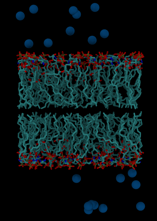
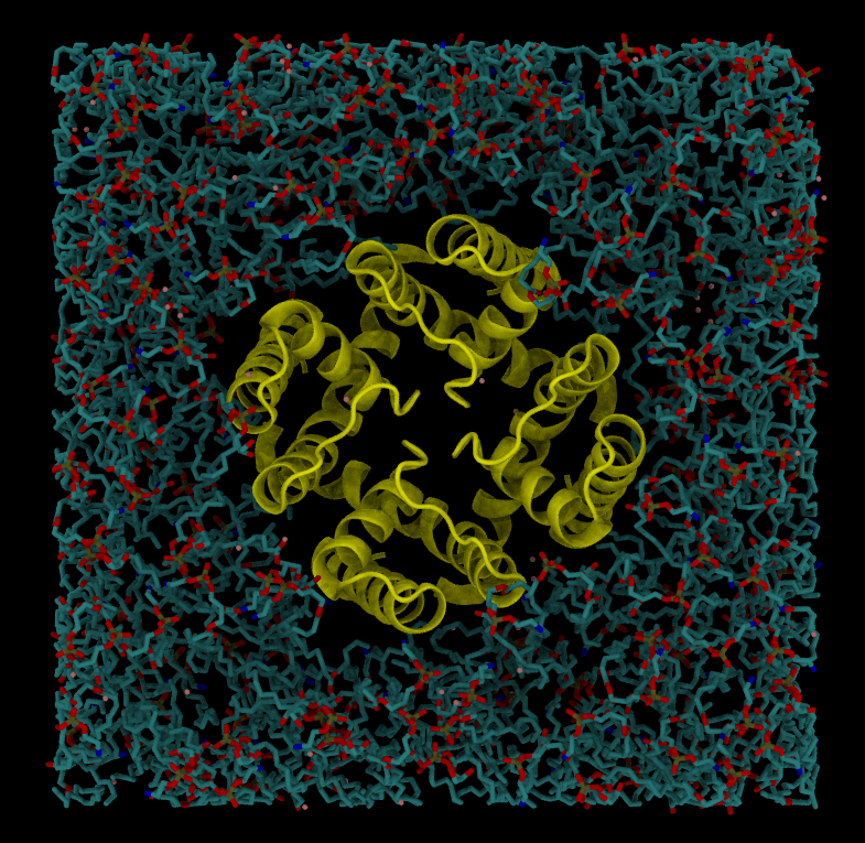
Embedding a protein into a bilayer
We will use PDB file 6U9P (wild-type MthK pore in ~150 mM K+) for this exercise.
- Use PPM server to orient a protein. PPM server will also take care of assembling the complete tetrameric pore.
- Use vmd to remove ligands and conformers B.
module purge
module load StdEnv/2023 vmd
vmd
mol new 6U9Pout.pdb
set sel [atomselect top "protein and not altloc B"]
$sel writepdb 6U9P-clean.pdb
quit
- Embed the protein into the lipid bilayer
 #!/bin/bash
 #SBATCH --mem-per-cpu=2000M
 #SBATCH --time=3:00:00

 module purge
 module load StdEnv/2023 ambertools/23
 packmol-memgen \
    --pdb 6U9P-clean.pdb \
    --lipids DOPE:DOPG \
    --ratio 3:1 \
    --preoriented \
    --parametrize
- To create topology.
--parametrize - The default protein force field is FF14SB, water model TIP3P
- To use a different force field:
--fprot ff19SB --ffwat opc --gaff2 - To add salt (default K+, 0.15M):
--salt - To make bilayer patch larger:
--dims 95 95 85
Links to advanced AMBER tutorials
- Placing waters and ions using 3D-RISM and MOFT
- Building a Membrane System with PACKMOL-Memgen
- Minimizing and Equilibrating a packed membrane system
- Setup and simulation of a membrane protein with AMBER Lipid21 and PACKMOL-Memgen.
Key Points
End of Workshop
Overview
Teaching: min
Exercises: minQuestions
Objectives
Key Points
Hands-on 1: Packing a complex mixture of different lipid species into a bilayer and simulating it
Overview
Teaching: 30 min
Exercises: 5 minQuestions
How to pack a complex mixture of different lipid species into a bilayer?
How to minimize energy?
How to heat up a simulation system?
How to equilibrate a simulation system?
Objectives
Prepare a lipid bilayer
Energy minimize, heat up and equilibrate the system
Introduction
This episode guides you through the process of building a bilayer, preparing simulation input files, minimizing energy, equilibrating the system, and running an equilibrium molecular dynamics simulation. You will need to follow a number of steps to complete the tutorial. If you are already familiar with some of these topics, you can skip them and focus on the ones you don’t know about.
1. Generating a bilayer by packing lipids together.
The packmol-memgen program allows the creation of asymmetric bilayers with leaflets composed of different lipid species.
Bilayer asymmetry is a common feature of biological membranes. For example, the composition of the phospholipids in the erythrocyte membrane is asymmetric. Here is an article that reviews this topic in detail: Interleaflet Coupling, Pinning, and Leaflet Asymmetry—Major Players in Plasma Membrane Nanodomain Formation.
Asymmetric lipid bilayer can be generated by the following submission script:
#!/bin/bash
#SBATCH --mem-per-cpu=4000M
#SBATCH --time=1:00:00
#SBATCH --cpus-per-task=1

module purge
module load StdEnv/2020 gcc/9.3.0 openmpi/4.0.3 ambertools/23

rm -f bilayer* *.log
packmol-memgen \
    --lipids PSM:POPC:POPS:POPE//PSM:POPC:POPS:POPE \
    --salt --salt_c Na+ --salt_a Cl- --saltcon 0.25 \
    --dist_wat 25 \
    --ratio 21:19:1:7//2:6:15:25 \
    --distxy_fix 100 \
    --parametrize
The job takes about 30 minutes. It generates several output files:
- AMBER topology bilayer_only_lipids.top
- AMBER coordinates bilayer_only_lipids.crd
- PDB-formatted system bilayer_only_lipids.pdb
By default LIPID17, ff14SB and TIP3P force fields are used.
2. Using AMBER force fields not available natively in packmol-memgen.
Packmol-memgen offers several recent AMBER force fields that can be used to parameterize a bilayer. However, sometimes it is necessary to use force fields that are not readily available in packmol-memgen. The parameterization of a prepared bilayer with tleap directly is a way to achieve this. To use tleap you will need to provide an input file that is in pdb format compatible with AMBER.
Even though packmol-memgen creates a pdb file (bilayer_only_lipids.pdb), you should use it with caution. It may not work properly with some molecules. PSM is an example. When saving pdb file containing this type of lipids packmol-memgen erroneously adds TER record between the lipid headgroup (SPM) and second acyl tail (SA). This splits PSM molecule in two: PA+SPM and SA.
To illustrate the parameterization process, we will create a pdb file from AMBER topology and coordinate files, and then parameterize the bilayer using the polarizable water OPC3-pol not yet available natively in packmol-memgen.
Begin by loading the ambertools/23 module and starting the Python interpreter:
module load StdEnv/2020 gcc/9.3.0 openmpi/4.0.3 ambertools/23
python
In the python prompt enter the following commands:
import parmed
amber = parmed.load_file("bilayer_only_lipid.top", "bilayer_only_lipid.crd")
amber.save("bilayer-lipid21-opc3pol.pdb")
quit()
We only need to know one more thing before we can proceed: the dimensions of the periodic box. Box information can be extracted from the file bilayer_only_lipid.top:
grep -A2 BOX bilayer_only_lipid.top
...
%FORMAT (5E168)
  9.00000000E+01  1.03536600E+02  1.03744300E+02  9.97203000E+01
The last three numbers refer to the size of the box in the X, Y, and Z axes. We can now parameterize the system using the Lipid21 force field and OPC3-Pol polarizable water as follows:
module load StdEnv/2020 gcc/9.3.0 openmpi/4.0.3 ambertools/23
tleap -f <(cat << EOF
source leaprc.water.opc3pol
source leaprc.lipid21
sys=loadpdb bilayer-lipid21-opc3pol.pdb
set sys box {103.5 103.7 99.7}
set default nocenter on
saveamberparm sys bilayer.parm7 bilayer.rst7
quit
EOF)
Don’t forget to replace {103.5 103.5 99.9} with your own numbers!
3. Energy minimization
A system must be optimized in order to eliminate clashes and prepare it for molecular dynamics.
To run energy minimization we need three files:
- Molecular topology bilayer.parm7
- Initial coordinates bilayer.rst7
- Simulation input file minimization.in
First, we create a directory for energy minimization job.
mkdir 1-minimization && cd 1-minimization
Here is an input file for minimization (minimization.in) that you can use.
Minimization
 &cntrl
  imin=1,       ! Minimization
  ntmin=3,      ! Steepest Descent
  maxcyc=1000,  ! Maximum number of cycles for minimization
  ntpr=10,      ! Print to mdout every ntpr steps
  ntwr=1000,    ! Write a restart file every ntwr steps
  cut=10.0,     ! Nonbonded cutoff
 /
Using the script below, submit a minimization job.
#!/bin/bash
#SBATCH --mem-per-cpu=4000
#SBATCH --ntasks=10
#SBATCH --time=1:00:00

module purge
module load StdEnv/2020 gcc/9.3.0 openmpi/4.0.3 ambertools/23

srun sander.MPI -O -i minimization.in \
        -o minimization.out \
        -p ../bilayer.parm7 \
        -c ../bilayer.rst7 \
        -r minimized.rst7
When the optimization job is completed, the output file minimized.rst7 will contain the optimized coordinates. Minimization takes about 40 minutes.
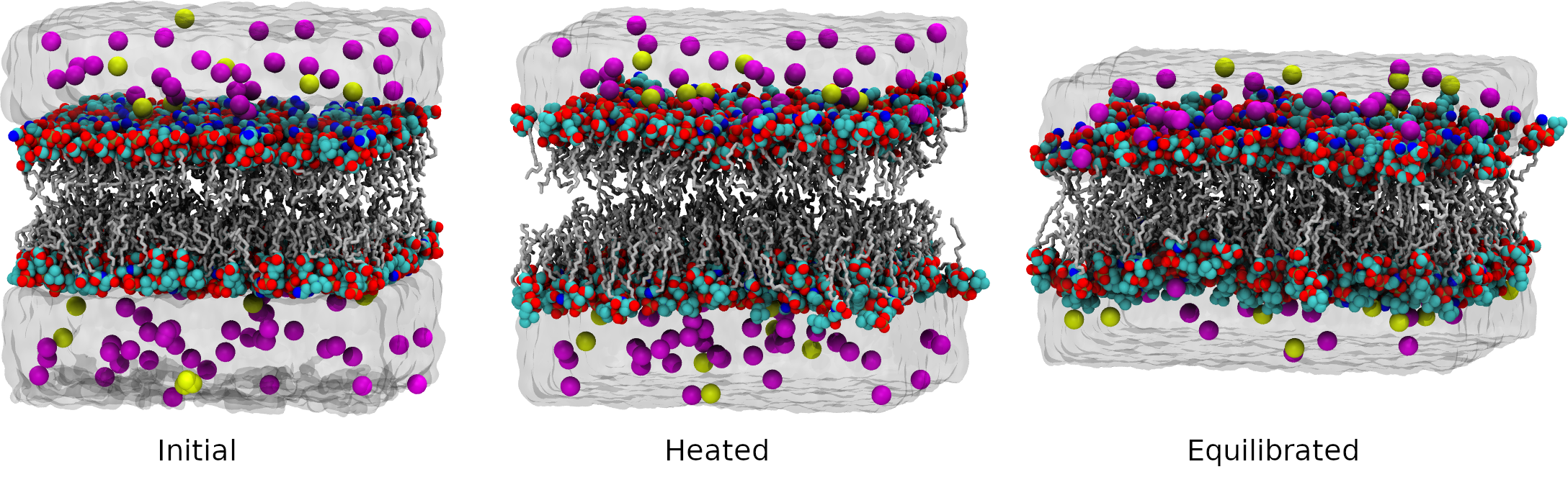
4. Heating
Start with creating a directory for energy heating job.
cd ..
mkdir 2-heating && cd 2-heating
Our optimized simulation system does not move yet, there is no velocities. Our next step is to heat it up to room temperature. The system can be heated in a variety of ways with different initial temperatures and heating rates. It’s important to warm up the system gently, avoiding strong shocks that can create conformations that aren’t physiological. A typical protocol is described in Amber tutorial Relaxation of Explicit Water Systems.
We will start the system at the low temperature of 100K and heat it up to 300K over 20 ps of simulation time at constant pressure. At this step we use weak coupling thermostat and barostat with both time constants set to 5 ps.
Here is how the simulation input file heating.in looks like:
Heating
 &cntrl
  imin=0,           ! Molecular dynamics
  ntx=1,            ! Read coordinates with no initial velocities
  ntc=2,            ! SHAKE on for bonds with hydrogen
  ntf=2,            ! No force evaluation for bonds with hydrogen
  tol=0.0000001,    ! SHAKE tolerance
  nstlim=20000,     ! Number of MD steps
  ntt=1,            ! Berendsen thermostat
  tempi=100,        ! Initial temperature
  temp0=300,        ! Target temperature
  tautp=5.0,        ! Time constant for heat bath coupling
  ntpr=100,         ! Write energy info every ntwr steps
  ntwr=10000,       ! Write restart file every ntwr steps
         ntwx=2000,        ! Write to trajectory file every ntwx steps
  dt=0.001,         ! Timestep
  ntb=2,            ! Constant pressure periodic bc.
  barostat=1,       ! Berendsen barostat
  taup=5,           ! Pressure relaxation time
  ntp=3,            ! Semiisotropic pressure scaling
  csurften=3,       ! Constant surface tension with interfaces in the xy plane
  cut=10.0,         ! Nonbonded cutoff
 /
Submit job using the following script:
#!/bin/bash
#SBATCH --mem-per-cpu=4000M
#SBATCH --gpus-per-node=v100:1
#SBATCH --time=1:00:00

module purge
module load StdEnv/2020 gcc/9.3.0 cuda/11.4 openmpi/4.0.3 amber/20.12-20.15

pmemd.cuda -O -i heating.in \
    -o heating.out \
    -p ../bilayer.parm7 \
    -c minimized.rst7 \
    -r heated.rst7
A minute is all it takes for this job to be completed.
5. The first phase of the equilibration process.
The second step of relaxation will maintain the system at 300 K over 100 ps of simulation time at a constant pressure, allowing the box density to relax. The initial density is too low because there are gaps between lipids an water and lipids are not perfectly packed.
As the simulation parameters are the same as on the previous step, you might wonder why we did not simply continue with the previous step? It is necessary to restart because the box size changes rapidly from its original size, and a running simulation cannot handle such large changes (GPU code does not reorganize grid cells at runtime). Restarting simulation will generate new grid cells and allow the simulation to continue.
Simulation input file equilibration.in:
Equilibration 1
 &cntrl
  imin=0,           ! Molecular dynamics
  irest=1,          ! Restart
  ntx=5,            ! Read positions and velocities
  ntc=2,            ! SHAKE on for bonds with hydrogen
  ntf=2,            ! No force evaluation for bonds with hydrogen
  tol=0.0000001,    ! SHAKE tolerance
  nstlim=200000,    ! Number of MD steps
  ntt=1,            ! Berendsen thermostat
  temp0=300,        ! Set temperature
  tautp=5.0,        ! Time constant for heat bath coupling
  ntpr=100,         ! Write energy info every ntwr steps
  ntwr=10000,       ! Write restart file every ntwr steps
  ntwx=2000,        ! Write to trajectory file every ntwx steps
  dt=0.001,         ! Timestep (ps)
  ntb=2,            ! Constant pressure periodic bc.
  barostat=1,       ! Berendsen barostat
  taup=5,           ! Pressure relaxation time
  ntp=3,            ! Semiisotropic pressure scaling
  csurften=3,       ! Constant surface tension with interfaces in the xy plane
  fswitch=8.0,      ! Force switching
  cut=10.0,         ! Nonbonded cutoff
 /
Submission script
#!/bin/bash
#SBATCH --mem-per-cpu=4000M
#SBATCH --gpus-per-node=v100:1
#SBATCH --time=1:00:00

module purge
module load StdEnv/2020 gcc/9.3.0 cuda/11.4 openmpi/4.0.3 amber/20.12-20.15

pmemd.cuda -O -i equilibration.in \
    -o eq-1.out \
    -p ../bilayer.parm7 \
    -c ../2-heating/heated.rst7 \
    -r eq-1.rst7
This job completes in about 5 minutes.
Examine energy components
log=eq-1.out
cpptraj << EOF
readdata $log
writedata energy.dat $log[Etot] $log[TEMP] $log[PRESS] $log[VOLUME] time 0.1
EOF
6. The second phase of the equilibration process.
Now density is mostly relaxed and we can apply temperature and pressure coupling parameters appropriate for a production run. Temperature and pressure coupling methods are changed to produce the correct NPT ensemble. To speed up simulation, we use a longer time step. The relaxation of a bilayer may take many nanoseconds. We simulate only for 1,000,000 steps because box dimensions are still far from equilibration and restart will likely be necessary to reorganize grid cells.
Simulation input file equilibration-2.in:
Equilibration 2
 &cntrl
  imin=0,           ! Molecular dynamics
  irest=1           ! Restart
  ntx=5,            ! Read  positions and  velocities
  ntc=2,            ! SHAKE on for bonds with hydrogen
  ntf=2,            ! No force evaluation for bonds with hydrogen
  tol=0.0000001,    ! SHAKE tolerance
  nstlim=1000000,   ! Number of MD steps
  ntt=3,            ! Langevin thermostat
  temp0=300,        ! Target temperature
  gamma_ln=2.0,     ! Collision frquency
  ntpr=100,         ! Write energy info every ntwr steps
  ntwr=10000,       ! Write restart file every ntwr steps
  ntwx=10000,       ! Write to trajectory file every ntwx steps
  dt=0.002,         ! Timestep (ps)
  ntb=2,            ! Constant pressure periodic bc.
  barostat=1,       ! Berendsen barostat
  taup=1.0,         ! Pressure relaxation time
  ntp=3,            ! Semiisotropic pressure scaling
  csurften=3,       ! Constant surface tension with interfaces in the xy plane
  fswitch=10.0,     ! Force switching from 10 to 12 A
  cut=12.0,         ! Nonbonded cutoff
 /
Submission script
#!/bin/bash
#SBATCH --mem-per-cpu=4000M
#SBATCH --gpus-per-node=v100:1
#SBATCH --time=6:00:00

module purge
module load StdEnv/2020 gcc/9.3.0 cuda/11.4 openmpi/4.0.3 amber/20.12-20.15

pmemd.cuda -O -i equilibration-2.in \
    -o eq-2.out \
    -p ../bilayer.parm7 \
    -c ../3-equilibration/eq-1.rst7 \
    -r eq-2.rst7
Center trajectory using the bilayer COM
trajin ../bilayer.rst7
trajin ../2-heating/heated.rst7
trajin ../4-equilibration/eq-4.rst7
center :SPM,PA,PC,PS
image
trajout mdcrd.xtc
go
quit
Delete TER records between residues SPM and SA in bilayer_only_lipid.pdb using shell commands.
This exercise is optional for those who wish to improve their efficiency when working with text files. Using shell commands at an advanced level is the focus of the exercise.
Solution
The following command removes all erroneous TER records:
grep -n  "H22 SPM " bilayer_only_lipid.pdb | \
 cut -f1 -d: | \
 awk '{print $0 + 1}' | \
 awk -F, 'NR==FNR { nums[$0]; next } !(FNR in nums)' \
 - bilayer_only_lipid.pdb > bilayer_only_lipid_fixed.pdb
Let’s break it down:
grep -n "H22 SPM "finds all lines containing “H22 SPM “ and prints their line numbers followed by the line content.cut -f1 -d:selects the first field containing the line numberawk '{print $0 + 1}increments this number, after this command we have a list of lie numbers we want to deleteawk -F, 'NR==FNR { nums[$0]; next } !(FNR in nums)' - bilayer_only_lipid.pdbtakes the list of line numbers from the pipe and deletes lines with matching numbers from the file bilayer_only_lipid.pdbIf this command is executed, it will remove the line following the last atom of each SPM residue, effectively deleting the erroneous TER records.
Key Points
Hands-on 2: Transferring AMBER simulation to GROMACS
Overview
Teaching: 20 min
Exercises: 5 minQuestions
How to use GROMACS to continue a simulation equilibrated with AMBER?
Objectives
Restart a running AMBER simulation with GROMACS
Moving simulations from AMBER to GROMACS
A specific MD software may provide you with a method that you cannot find in other software. What to do if you already have prepared and equilibrated a simulation? MD packages are reasonably compatible with each other, which makes transferring simulations possible. During this hands-on activity, you will transfer the equilibrated bilayer simulation you prepared in hands-on 1 to GROMACS.
Typically GROMACS simulations are restarted from checkpoint files in cpt format. By default, GROMACS writes a checkpoint file of your system every 15 minutes.AMBER restart files cannot be used to create a GROMACS checkpoint file, so we will prepare a GROMACS run input file (tpr).
- Change directory to 4-equilibration.
- Create a directory for GROMACS simulation
- Load ambertools and gromacs modules and start python
mkdir 5-amb2gro && cd 5-amb2gro
module load StdEnv/2020 gcc/9.3.0 openmpi/4.0.3 ambertools/23 gromacs/2023.2
python
Converting AMBER restart and topology to GROMACS.
Using parmed, convert AMBER topology and restart files to GROMACS.
import parmed as pmd
amber = pmd.load_file("../bilayer.parm7", "../4-equilibration/eq-2.rst7")
ncrest=pmd.amber.Rst7("../4-equilibration/eq-2.rst7")
amber.velocities=ncrest.vels
amber.save("restart.gro")
amber.save("bilayer.top")
quit()
These parmed commands will create two GROMACS files: restart.gro (coordinates and velocities) and bilayer.top.
Creating and editing index file
The default index file can be created using the command:
gmx make_ndx -f restart.gro
It has 13 groups:
...
  0 System              : 113855 atoms
  1 Other               : 47155 atoms
  2 PA                  : 16882 atoms
  3 SPM                 :  3441 atoms
  4 SA                  :  4092 atoms
  5 PC                  :  3762 atoms
  6 OL                  : 13700 atoms
  7 PE                  :  3422 atoms
  8 PS                  :  1767 atoms
  9 Na+                 :    73 atoms
 10 Cl-                 :    16 atoms
 11 Water               : 66700 atoms
 12 SOL                 : 66700 atoms
 13 non-Water           : 47155 atoms
...
Groups SOL and non-Water can be deleted. There will be two thermostats: one thermostat will be used for lipids, and another one for everything else. For these thermostats we have to create two new groups: Lipids and Water+Ions.
Here are the commands to do it:
gmx make_ndx -f restart.gro << EOF
del 12
del 12
1&!rNa+&!rCl-
name 12 Lipids
11|rNa+|rCl-
name 13 WaterIons
q
EOF
Check created index file:
gmx make_ndx -f restart.gro -n index.ndx
You should have two new groups:
12 Lipids              : 53850 atoms
13 WaterIons           : 66792 atoms
As packing bilayer and solvating it is non-deterministic, the number of atoms may be slightly different in your case.
Creating a portable binary run input file.
GROMACS run input files (.tpr) contain everything needed to run a simulation: topology, coordinates, velocities and MD parameters.
gmx grompp -p bilayer.top -c restart.gro -f production.mdp -n index.ndx -maxwarn 1
GROMACS simulation input file production.mdp
Title                   = bilayer
; Run parameters
integrator              = md
nsteps                  = 400000
dt                      = 0.001
; Output control
nstxout                 = 0
nstvout                 = 0
nstfout                 = 0
nstenergy               = 100
nstlog                  = 10000
nstxout-compressed      = 5000
compressed-x-grps       = System
; Bond parameters
continuation            = yes
constraint_algorithm    = lincs
constraints             = h-bonds
; Neighborsearching
cutoff-scheme           = Verlet
ns_type                 = grid
nstlist                 = 10
rcoulomb                = 1.0
rvdw                    = 1.0
DispCorr                = Ener ; anaytic VDW correction
; Electrostatics
coulombtype             = PME
pme_order               = 4
; Temperature coupling is on
tcoupl                  = V-rescale
tc-grps                 = WaterIons Lipids
tau_t                   = 0.1 0.1
ref_t                   = 300 300
; Pressure coupling is on
pcoupl                  = Parrinello-Rahman
pcoupltype              = semiisotropic
tau_p                   = 5.0
ref_p                   = 1.0 1.0
compressibility         = 4.5e-5 4.5e-5
; Periodic boundary conditions
pbc                     = xyz
; Velocity generation
gen_vel                 = no
Running GROMACS simulation
#!/bin/bash
#SBATCH --mem-per-cpu=4000M
#SBATCH --time=1:00:00
#SBATCH --cpus-per-task=10
#SBATCH --gpus-per-node=v100:1

module load StdEnv/2020 gcc/9.3.0 cuda/11.4 openmpi/4.0.3 gromacs/2023.2

srun gmx mdrun -ntomp ${SLURM_CPUS_PER_TASK:-1} \
          -nb gpu -pme gpu -update gpu -bonded cpu -s topol.tpr
Key Points
Hands-on 3A: Preparing a Complex RNA-protein System
Overview
Teaching: 30 min
Exercises: 5 minQuestions
How to add missing segments to a protein?
How to add missing segments to a nucleic acid?
How to align molecules with VMD?
Objectives
?
Introduction
In this lesson, we will prepare simulation of a complex of human argonaute-2 (hAgo2) protein with a micro RNA bound to a target messenger RNA (PDBID:6N4O).
Micro RNAs (miRNAs) are short non-coding RNAs that are critical for regulating gene expression and the defense against viruses. miRNAs regulate a wide variety of human genes. They can control the production of proteins by targeting and inhibiting mRNAs. miRNAs can specifically regulate individual protein’s expression, and their selectivity is based on sequence complementarity between miRNAs and mRNAs. miRNAs that target messenger RNAs (mRNAs) encoding oncoproteins can serve as selective tumor suppressors. They can inhibit tumor cells without a negative impact on all other types of cells. The discovery of this function of miRNAs has made miRNAs attractive tools for new therapeutic approaches. However, it is challenging to identify the most efficient miRNAs that can be targeted for medicinal purposes. To regulate protein synthesis miRNAs interact with hAgo2 protein forming the RNA-induced silencing complex that recognizes and inhibits the target mRNAs by slicing them. Therefore, elucidating the structural basis of the molecular recognition between hAgo2 and mRNA is crucial for understanding miRNA functions and developing new therapeutics for diseases.
Create working directory:
mkdir ~/scratch/workshop/pdb/6N4O
cd ~/scratch/workshop/pdb/6N4O
1. Preparing a protein for molecular dynamics simulations.
1.1 Adding missing residues to protein structure files.
1.1.1 What residues are missing?
Almost all protein and nucleic acid crystallographic structure files are missing some residues. The reason for this is that the most flexible parts of biopolymers are disordered in crystals, and if they are disordered the electron density will be weak and fuzzy and thus atomic coordinates cannot be accurately determined. These disordered atoms, however, may be crucial for MD simulations (e.g., loops connecting functional domains, nucleic acid chains, incomplete amino acid side chains … etc.). For realistic simulation, we need to build a model containing all atoms.
How can we find out if any residues are missing in a PDB file? Missing residues, and other useful information is available in PDB file REMARKS. There are many types of REMARKS. The REMARK 465 lists the residues that are present in the SEQRES records but are completely absent from the coordinates section. You can find information about all types of REMARKS here.
Let’s see if our PDB file is missing any residues
grep "REMARK 465" ../6n4o.pdb | less
REMARK 465 MISSING RESIDUES
REMARK 465 THE FOLLOWING RESIDUES WERE NOT LOCATED IN THE
REMARK 465 EXPERIMENT. (M=MODEL NUMBER; RES=RESIDUE NAME; C=CHAIN
REMARK 465 IDENTIFIER; SSSEQ=SEQUENCE NUMBER; I=INSERTION CODE.)
REMARK 465
REMARK 465   M RES C SSSEQI
REMARK 465     MET A     1
REMARK 465     TYR A     2
REMARK 465     SER A     3
REMARK 465     GLY A     4
REMARK 465     ALA A     5
REMARK 465     GLY A     6
REMARK 465     PRO A     7
...
Yes, there is a bunch of missing residues, and we need to insert them to complete the model. One way to do this is to use homology modeling servers. Let’s use the SWISS-MODEL server.
1.1.2 Prepare a structural template and a sequence of the complete protein.
To add missing residues we need to supply a structure file with missing protein residues and a sequence of the complete protein. Let’s prepare these two required files.
Download structure and sequence files from PDB database:
wget https://files.rcsb.org/download/6n4o.pdb
wget https://www.rcsb.org/fasta/entry/6N4O/download -O 6n4o.fasta
Examine visually the file “6n4o.fasta”. There are sequences for 3 chains (A,C,D), each printed in one line. We will need a separate sequence file for each chain. Extract the complete sequences of the protein (chain A), and of the RNA (chains C,D). We will need them later. Can we use grep? We used grep to find a pattern in a file and print out the line containing this sequence. Can we ask grep to print the next line as well? Yes, there is an option -A for this!
grep -A1 "Chain A" 6n4o.fasta > 6n4o_chain_A.fasta
grep -A1 "Chain C" 6n4o.fasta > 6n4o_chain_C.fasta
grep -A1 "Chain D" 6n4o.fasta > 6n4o_chain_D.fasta
Use grep manual to see the meaning of the -A option.
Extract chain A from 6n4o.pdb using VMD
module load StdEnv/2020 gcc vmd
vmd
In the VMD console, execute the following commands:
mol new 6n4o.pdb
set sel [atomselect top "chain A"]
$sel writepdb 6n4o_chain_A.pdb
quit
1.1.3 Adding missing residues using the SWISS-MODEL server
Download 6n4o_chain_A.pdb and 6n4o_chain_A.fasta to your computer for homology modeling with SWISS-MODEL. You can do it with the scp program from your local computer:
- In a browser on your local computer navigate to SWISS-MODEL website.
- Click Start Modelling,
- Click User Template,
- Paste the full sequence of your protein or upload 6n4o_chain_A.fasta,
- Upload your structure file 6n4o_chain_A.pdb missing residues,
- Click Build Model
The workshop data already has this protein model in the directory “workshop/pdb/6N4O/protein_models”.
Are all missing residues added?
This protein model is in the directory “pdb/6N4O/protein_models”, in the file 6N4O_SWISS_PROT_model_chainA.pdb. How many residues should the complete model have? How many residues are in the file?
Solution
The complete Ago-2 protein has 859 residue, the model has 838. The first 21 residues are missing.
1.1.4 Adding missing residues using the i-TASSER server
The limitation of SWISS-MODEL server is that it is not capable of modeling long terminal fragments. Another homology modeling server i-TASSER (Iterative Threading ASSEmbly Refinement) uses the advanced protocol and is capable of predicting folding without any structural input. The downside of i-TASSER is that the process is much longer (about 60 hours for protein like 6n4o). We can not wait for i-TASSER modeling to complete, but the result is available in the workshop data tarball. Another drawback is that i-TASSER optimizes, positions of all atoms, which is great, but not always desirable.
1.2. Aligning protein models.
i-TASSER modeling procedure changes the orientation of the protein and slightly optimizes the positions of all atoms. We want keep the original atom positions, and only add the model of the N-terminal end. To combine the i-TASSER model with the actual 6n4o coordinates, we need to align the i-TASSER model with the original structure.
It is often very useful to align several structures for comparison. However, if a structure that you want to compare with the reference has a different number of residues or some deletions/insertions it is not straightforward to do an alignment. You will need to prepare two lists of structurally equivalent atoms.
We have two models of out protein in the directory.
cd ~/scratch/workshop/pdb/6N4O/protein_models
ls *model*
6N4O_i-TASSER_model_chainA.pdb 6N4O_SWISS_PROT_model_chainA.pdb
For alignment we want to use only the real data, the residues that are resolved in the crystallographic structure and are given in the PDB entry 6N4O. Let’s print out the list of missing residues again:
grep "REMARK 465" ../6n4o.pdb | less
Using this information we can compile a list of all residues that have coordinates. We will need this list for several purposes, such as alignment of protein molecules and constraining them during energy minimization and energy equilibration.
To begin the alignment process start VMD and load two pdb files. They will be loaded as molecules 0 and 1, respectively:
mol new 6N4O_SWISS_PROT_model_chainA.pdb
mol new 6N4O_i-TASSER_model_chainA.pdb
Define the the variable 6n4o_residues containing the list of all residues present in 6N4O.pdb:
set 6n4o_residues "22 to 120 126 to 185 190 to 246 251 to 272 276 to 295 303 to 819 838 to 858"
Select residues defined in the variable 6n4o_residues from both models, and save selections in the variables swissmodel and itasser. We have now two sets of equivalent atoms.
set swissmodel [atomselect 0 "backbone and resid $6n4o_residues"]
set itasser [atomselect 1 "backbone and resid $6n4o_residues"]
Now we need to find a rigid body transformation from itasser to swissmodel. The measure VMD command can compute the transformation matrix. It can measure lot of other useful things, such as rmsd, surface area, hydrogen bonds, energy and much more. And of course it can do it for each frame of a trajectory. You can get help on all options by typing “measure” in VND console.
Compute the transformation (rotation + translation 4;3) matrix TransMat.
set TransMat [measure fit $itasser $swissmodel]
The matrix describes how to move itasser atoms so that they overlap the corresponding swissmodel atom. Once the matrix is computed all we need to do is to appy it to the whole itasser model.
Select all residues of molecule 1 and apply the transformation to the selection.
echo rmsd before fit = [measure rmsd $itasser $swissmodel]
set itasser_all [atomselect 1 "all"]
$itasser_all move $TransMat
echo rmsd after fit = [measure rmsd $itasser $swissmodel]
Select residues 1-21 from molecule 1 and save them in the file 6n4o_resid_1-21.pdb
set term [atomselect 1 "noh resid 1 to 21"]
$term writepdb 6n4o_resid_1-21.pdb
quit
Combine the i-TASSER model of residues 1-21 with the SWISS-MODEL.
grep -h ATOM 6n4o_resid_1-21.pdb 6N4O_SWISS_PROT_model_chainA.pdb > 6n4o_chain_A_complete.pdb
1.3. Mutating residues
PDB entry 6N4O is the structure of the catalytically inactive hAgo2 mutant D669A. To construct the active form, we need to revert this mutation. Let’s use pdb4amber utility to mutate ALA669 to ASP:
pdb4amber -i 6n4o_chain_A_complete.pdb -o 6n4o_chain_A_complete_A669D.pdb -m "669-ALA,669-ASP"
Verify the result:
grep 'A 669' 6n4o_chain_A_complete_A669D.pdb
ATOM   5305  N   ASP A 669     -19.332  25.617 -27.862  1.00  0.97         N
ATOM   5306  CA  ASP A 669     -18.951  24.227 -27.916  1.00  0.97         C
ATOM   5307  C   ASP A 669     -17.435  24.057 -28.043  1.00  0.97         C
ATOM   5308  O   ASP A 669     -16.661  25.018 -28.091  1.00  0.97         O
This works, but it is not very smart because the program simply renames ALA to ASP and deletes all atoms except the 4 backbone atoms. While leap will rebuild the sidechain, it will not ensure that it is added in the optimal conformation. You can do a better job manually if you preserve all common atoms. Many types of mutations are different only in 1-2 atoms.
Mutating residues with stream editor
Mutate ALA669 to ASP669 using stream editor (sed), and keeping all common atoms.
Solution
To mutate ALA669 to ASP669, we need to delete from ALA669 all atoms that are not present in ASP. Then change the residue name of ALA to ASP. Let’s begin by checking what atoms are present in residue 669:
grep 'A 669' 6n4o_chain_A_complete.pdbATOM 5161 N ALA A 669 -19.332 25.617 -27.862 1.00 0.97 N ATOM 5162 CA ALA A 669 -18.951 24.227 -27.916 1.00 0.97 C ATOM 5163 C ALA A 669 -17.435 24.057 -28.043 1.00 0.97 C ATOM 5164 O ALA A 669 -16.661 25.018 -28.091 1.00 0.97 O ATOM 5165 CB ALA A 669 -19.720 23.530 -29.053 1.00 0.97 CIf you are familiar with aminoacid structures, you remember that the alanine sidechain is made of only one beta carbon atom (CB). All amino acids except glycine have beta carbon as well. So there is nothing to delete. All we need to do is to change the resName of all five ALA atoms to ASP. You can do it using stream editor:
sed 's/ALA A 669/ASP A 669/g' 6n4o_chain_A_complete.pdb > 6n4o_chain_A_complete_A669D.pdbVerify the result:
grep 'A 669' 6n4o_chain_A_complete_A669D.pdbATOM 5161 N ASP A 669 -19.332 25.617 -27.862 1.00 0.97 N ATOM 5162 CA ASP A 669 -18.951 24.227 -27.916 1.00 0.97 C ATOM 5163 C ASP A 669 -17.435 24.057 -28.043 1.00 0.97 C ATOM 5164 O ASP A 669 -16.661 25.018 -28.091 1.00 0.97 O ATOM 5165 CB ASP A 669 -19.720 23.530 -29.053 1.00 0.97 C
The check_structure utility will do mutation with minimal atom replacement. It will also complete sidechain and check it for clashes. If modeller suite is installed it can also relax added sidechains.
source ~/env-biobb/bin/activate
check_structure -i 6n4o_chain_A_complete.pdb -o 6n4o_chain_A_complete_A669D.pdb mutateside --mut ala669asp
Verify the result:
grep 'A 669' 6n4o_chain_A_complete_A669D.pdb
Adding functionally important ions.
The catalytic site of hAgo2 is comprised of the four amino acids D597, E637, D669 and H807. It is known that hAgo2 requires a divalent metal ion near the catalytic site to slice mRNA. The 6n4o PDB file does not have this ion, but another hAgo2 structure, 4w5o, does.
Align 4w5o with 6n4o and save all MG ions in the file “4w5o_MG_ions.pdb” so that we will be able to add them later to our simulation. For alignment use the catalytic site residues D597, E637, D669 and H807.
Solution
Download 4w5o.pdb
cd ~/scratch/workshop/pdb/6N4O/protein_models
wget https://files.rcsb.org/download/4w5o.pdb
mv 4w5o.pdb ../
Align 4w5o with 6n4o, renumber and save MG ions.
mol new ../6n4o.pdb
mol new ../4w5o.pdb
set 6n4o [atomselect 0 "backbone and resid 597 637 669 807"]
set 4w5o [atomselect 1 "backbone and resid 597 637 669 807"]
set TransMat [measure fit $4w5o $6n4o]
echo rmsd before fit = [measure rmsd $6n4o $4w5o]
set 4w5o_all [atomselect 1 "all"]
$4w5o_all move $TransMat
echo rmsd after fit = [measure rmsd $6n4o $4w5o]
set mg [atomselect 1 "resname MG"]
$mg set resid [$mg get residue]
$mg writepdb 4w5o_MG_ions.pdb
quit
2. Adding missing segments to RNA structure files.
Inspection of the PDB file 6n4o shows that several nucleotides are missing in both RNA chains. The RNA model must be completed, and all RNA atoms placed at the appropriate positions before we can start simulations the system.
First, we need to create a PDB file containing all RNA atoms. At this initial step, we are not particularly concerned with the quality of the 3D structure because we will refine it later.
We can insert the missing residues using the freely available ModeRNA server or standalone ModeRNA software. The automatic process used by ModeRNA server moves residues adjacent to the inserted fragment. Changing atomic positions is not desirable because we want to keep all experimental coordinates. Besides, modeRNA server offers a limited set of options, and the output PDB files will need more processing to make them usable in the simulation. For these reasons, we will use the standalone modeRNA package. ModeRNA software is available on CC systems. If you are comfortable with installation of Python, you can install it on your computer as well.
2.1. Using modeRNA on CC systems.
ModeRNA is a python module. To install it we need to create a python virtual environment, and the install ModeRNA modue into the environment.
module load StdEnv/2016.4 python/2.7.14
virtualenv ~/env-moderna
source ~/env-moderna/bin/activate
pip install numpy==1.11.3 biopython==1.58 ModeRNA==1.7.1
Installation is required only once. When you login into your account next time you only need to activate the environment:
module load StdEnv/2016.4 python/2.7.14
source ~/env-moderna/bin/activate
Once you install modeRNA program, you will be able to use all its functions. As modeRNA inserts missing fragments only into a single RNA strand, we need to model chains C and D separately. For insertion of missing residues we need to prepare anstructural template and a sequence alignment file for each RNA strand.
2.2. Preparing a structural template for chains C and D.
Let’s go into the directory where we will be working with RNA models.
mkdir ~/scratch/workshop/pdb/6N4O/RNA_models/modeRNA
cd ~/scratch/workshop/pdb/6N4O/RNA_models/modeRNA
To make a structural template we will prepare a pdb file containing only RNA from 6n4o.pdb. One file containing both RNA chains (C and D) is sufficient.
module load StdEnv/2020 gcc vmd
vmd
mol new ../../6n4o.pdb
set sel [atomselect top "chain C or (chain D and not resid 6)"]
$sel writepdb 6n4o_chains_CD.pdb
quit
Because residue 6 in chain D has only phosphate atoms it cannot be used as a template, so we remove it.
We created the file 6n4o_chains_CD.pdb suitable for use as a structural template. Next, we need to prepare sequence alignment files for chains C and D. These files describe a sequence of the model to be built and a sequence matching the structural template where the missing residues to be inserted are represented with ‘-‘.
2.4. Preparing sequence alignment files for chains C and D.
What residues are missing?
grep "REMARK 465" ../6n4o.pdb
...
REMARK 465       A C    10
REMARK 465       U C    19
REMARK 465       U D     7
REMARK 465       C D     8
REMARK 465       A D    17
REMARK 465       A D    18
Copy RNA fasta files into the current directory (~/scratch/workshop/pdb/6N4O/RNA_models/modeRNA)
cp ../../6n4o_chain_C.fasta ../../6n4o_chain_D.fasta .
Use a text editor of your choice (for example, nano or vi) to edit these two sequence alignment files. Each file must contain two sequences, the sequence of the model to be built and the template sequence matching the structural template. The contents of the files is shown below.
Sequence alignment file for chain C:
cat 6n4o_chain_C.fasta
>Model
UGGAGUGUGACAAUGGUGUUU
>Template
UGGAGUGUG-CAAUGGUG-UU
Sequence alignment file for chain D:
cat 6n4o_chain_D.fasta
>Model
CCAUUGUCACACUCCAAA
>Template
CCAUU---ACACUCCA--
2.5. Inserting missing segments.
Below are the commands needed to insert missing fragments in chains C and D. The detailed description of all modeRNA commands is available here.
from moderna import *
# Model chain C
tC = load_template('6n4o_chains_CD.pdb', 'C')  # template C
aC = load_alignment('6n4o_chain_C.fasta')      # alignment C
mC = create_model(model_chain_name = 'A')      # model C
apply_alignment(tC, aC, mC)
apply_indel(mC, '9', '11', 'A')  # insert A between 9 and 11
apply_indel(mC, '18', '20', 'U') # insert U between 18 and 20
renumber_chain(mC, '1')
write_model(mC, 'chain_C_model_A.pdb')
# Model chain D
tD = load_template('6n4o_chains_CD.pdb', 'D')
aD = load_alignment('6n4o_chain_D.fasta')
mD = create_model(model_chain_name = 'B')
apply_alignment(tD, aD, mD)
apply_indel(mD, '5', '9', 'GUC')
apply_missing_ends(aD, mD)
renumber_chain(mD, '1')
write_model(mD, 'chain_D_model_B.pdb')
Start python and execute the commands interactively:
module --force purge
module load StdEnv/2016.4 python/2.7.14
source ~/env-moderna/bin/activate
python
Or save these commands in the file make_models.py and run it non-iteractively.
The modeRNA program will create two model files, chain_C_model_A.pdb, and chain_D_model_B.pdb. Ensure that the program added all missing residues and did not move any residues present in the original structure file.
How will ModeRNA server do the same task?
Try using ModeRNA server. Compare automatically generated ModeRNA models with the original chains C and D. Did server only add missing residues without moving any other atoms? Can you spot any other pitfalls with the automatically generated models?
Solution
ModeRNA server inserts missing residues with the same residue number as the residue before insertion. It uses an insertion code (iCode) to mark inserted residues. For example, if residues 6-8 are missing, the program will insert them as residues 5A, 5B, and 5C. It is not possible to instruct ModeRNA webserver to renumber residues, and it is not possible to change chainID either. So you will need to take care of residue numbering and renaming chains manually.
References:
3. Optimizing double stranded RNA.
As we built two complementary RNA strands independently of each other, they clash when two strands are combined.
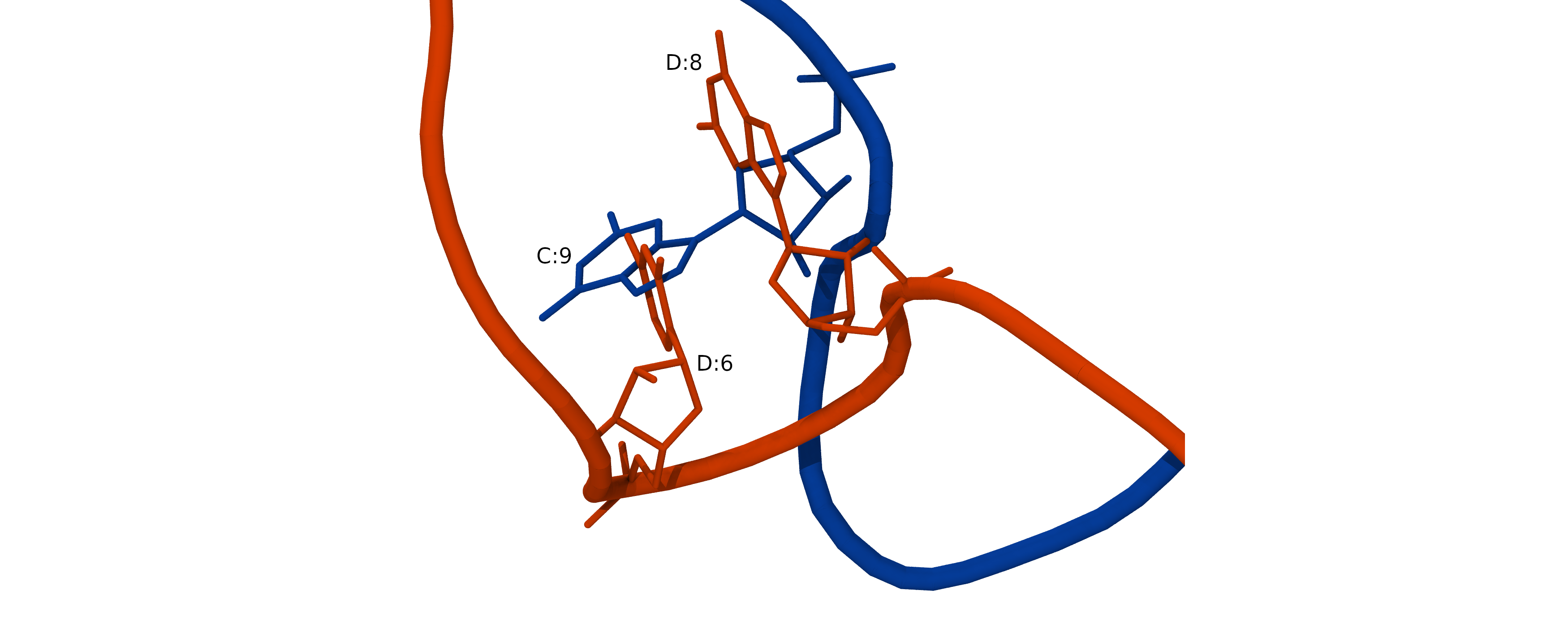
To resolve steric clashes and obtain a good initial RNA structure, we need to optimize the whole RNA duplex. We will use a Monte-Carlo based simulation program SimRNA. It is available as SimRNAweb server or standalone SimRNA software. This program allows for RNA 3D structure modeling with optional restraints.
SimRNA features:
- Coarse-grained representation (5 atoms per residue)
- Monte Carlo method for sampling the conformational space
- The energy function is composed of statistical potential terms, derived from the observed frequencies of occurrence of various proximate structural patterns.
3.1. Download and unpack SimRNA binary package:
Simulation submitted to public SimRNAweb server may wait up to a few days in the queue, while on a local computer, you can do it in a couple of minutes. SimRNA is available as a binary distribution, so no installation is required. You only need to download and unpack the package:
mkdir ~/scratch/workshop/pdb/6N4O/RNA_models/simRNA
cd ~
wget https://ftp.users.genesilico.pl/software/simrna/version_3.20/SimRNA_64bitIntel_Linux.tgz --no-check-certificate
tar -xf SimRNA_64bitIntel_Linux.tgz
cd ~/scratch/workshop/pdb/6N4O/RNA_models/simRNA
Preparing input files for simulation with SimRNAweb server.
If you will be using standalone SimRNA program you can skip this section and proceed to the next one.
SimRNAweb server requires RNA sequence, a list of residues not allowed to move in simulation, and RNA structure in PDB format.
RNA sequence:
UGGAGUGUGACAAUGGUGUUU CCAUUGUCACACUCCAAAA list of residues not allowed to move (we don’t want the program to move atoms resolved in the experimental structure).
A:1-9,11-18,20-21;B:1-5,9-16PDB file matching the sequence. All atoms must be present, and chains must be named A and B. To prepare this file combine the model of chain C, the 5’ phosphate from chain_D_model_B5P.pdb, and the model of chain D. Change the residue name to C5 and chain ID to B for the phosphate atoms.
cat chain_C_model_A.pdb > chains_CD_model_AB.pdb
head -n 4 chain_D_model_B5P.pdb | sed 's/C5   /  C B/g' >> \
chains_CD_model_AB.pdb
cat chain_D_model_B.pdb >> chains_CD_model_AB.pdb
3.2. Preparing a simulation with a standalone version of SimRNA.
For simulation with SimRNA you will need to modify the PDB structure file. Command-line SimRNA program does not take a list of frozen atoms as a separate input. Instead, you need to give this information in the occupancy field of the PDB structure file. But before we flag frozen atoms the missing phosphate must be added to the 5’ terminal residue of chain D.
We begin with merging models of chains A and B if you have not done this yet:
mkdir ~/scratch/workshop/pdb/6N4O/RNA_models/simRNA
cd ~/scratch/workshop/pdb/6N4O/RNA_models/simRNA
cat ../modeRNA/chain_C_model_A.pdb ../modeRNA/chain_D_model_B.pdb > chains_CD_model_AB.pdb
Next, we apply two modifications to this file. First, we need to add phosphate to the 5’ terminal residue of chain D. SimRNA expects all residues to have a P atom. SimRNAweb will add P automatically, but for simulation with a standalone SimRNA program, we need to do it manually. There are several options to add the phosphate.
3.2.1. Renaming O5’ atom to P
The most straightforward fix is to rename O5’ atom to P. if you chose to do this, save the edited file chains_CD_model_AB.pdb as chains_CD_model_AB_5P.pdb, and skip the next step.
3.2.2. Adding 5’ monophosphate with AmberTools/20.
First, rename the phosphorylated 5’ terminal nucleotide C according to AMBER convention to C5. The names of phosphorylated terminals in AMBER are A5, C5, G5, U5, DA5, DC5, DG5, and DT5. The libraries of phosphorylated 5’ terminal nucleotides are in the file ‘$AMBERHOME/dat/leap/lib/terminal_monophosphate.lib’.
module purge
module load gcc/9.3.0 cuda/11.4  ambertools/22
Launch Leap and load RNA force field:
tleap -f leaprc.RNA.OL3 -I $EBROOTAMBERTOOLS/dat/leap/lib/
In the Leap promt execute the commands:
loadoff terminal_monophosphate.lib
chainD = loadpdb chain_D_model_B.pdb
savepdb chainD chain_D_model_B5P.pdb
quit
These commands will load libraries of phosphorylated 5’ terminal nucleotides and chain D PDB file. Leap will automatically add all missing atoms based on library entries and save chainD in the PDB file chain_D5P.pdb:
We don’t want to use the PDB file prepared with Leap for SimRNA because AMBER has different aminoacid naming conventions. So we copy phosphate atoms from chain_D5P.pdb and paste them into chains_CD_model_AB.pdb. We then edit chain ID, residue ID, and residue name. Save the edited file chains_CD_model_AB.pdb as chains_CD_model_AB_5P.pdb
3.2.3. Adding 5’ mono-phosphate with CHARMM-GUI.
You can also add phosphate using CHARMM-GUI. Beware that CHARMM-GUI changes residue names to the old-style RNA 3-letter names and changes chain ID to “R”.
3.2.4 Define frozen atoms.
Standalone SimRNA program accepts PDB file where frozen atoms have occupancy 0.0 and completely free have occupancy 1.0. You can change values of the occupancy with the following VMD commands:
module --force purge
module load StdEnv/2020 gcc vmd
vmd
mol new chains_CD_model_AB_5P.pdb
set sel [atomselect top all]
$sel set occupancy 0
set sel [atomselect top "chain A and resid 10 19"]
$sel set occupancy 1
set sel [atomselect top "chain B and resid 6 7 8 17 18"]
$sel set occupancy 1
set sel [atomselect top all]
$sel writepdb chains_CD_model_AB_5P_frozen.pdb
quit
3.3. Running simulation
SimRNA needs two files in the working directory:
- chains_CD_model_AB_5P_frozen.pdb, pdb file with flagged frozen atoms
- config, the file with SimRNA simulation parameters.
Example configuration file:
NUMBER_OF_ITERATIONS 1000000
TRA_WRITE_IN_EVERY_N_ITERATIONS 10000
INIT_TEMP 1.35
FINAL_TEMP 0.90

BONDS_WEIGHT 1.0
ANGLES_WEIGHT 1.0
TORS_ANGLES_WEIGHT 0.0
ETA_THETA_WEIGHT 0.40
In the working directory, make a symbolic link to the ‘data’ directory located in SimRNA distribution. Assuming that you installed SimRNA in $HOME the link command is:
cd ~/scratch/workshop/pdb/6N4O/RNA_models/simRNA
ln -s ~/SimRNA_64bitIntel_Linux/data data
Then run the simulation:
srun -c2 --mem-per-cpu=1000 --time=30:0 \
~/SimRNA_64bitIntel_Linux/SimRNA \
-P chains_CD_model_AB_5P_frozen.pdb \
-c config -E 2
The option -E <number of replicas> turns on replica exchange mode. Replica exchange mode is parallelized with OMP. Each replica simulation can run on its own CPU independently of others, so for the optimal performance allocate the same number of cores (option -c) as the number of replicas (option -E).
The simulation will run for about two minutes and produce trajectory file *.trafl for each replica.
3.4. Processing simulation trajectory
The simplest way of processing the trajectory files is obtaining the lowest energy structure. Generally, better results can be obtained by using clustering. Clustering tool is included with the distribution, but using clustering is outside the scope of this workshop.
Extract the lowest energy frame from the trajectory of the first replica
~/SimRNA_64bitIntel_Linux/trafl_extract_lowestE_frame.py \
chains_CD_model_AB_5P_frozen.pdb_01.trafl
Convert the lowest energy frame to PDB format
~/SimRNA_64bitIntel_Linux/SimRNA_trafl2pdbs chains_CD_model_AB_5P.pdb \
chains_CD_model_AB_5P_frozen.pdb_01_minE.trafl 1 AA
This command will create PDB file of the lowest energy structure from trajectory of replica 1: chains_CD_model_AB_5P_frozen.pdb_01_minE-000001_AA.pdb We will use this relaxed structure for simulation. Rename it into a shorter name, for example chains_CD_minimized.pdb
cp chains_CD_model_AB_5P_frozen.pdb_01_minE-000001_AA.pdb chains_CD_minimized.pdb
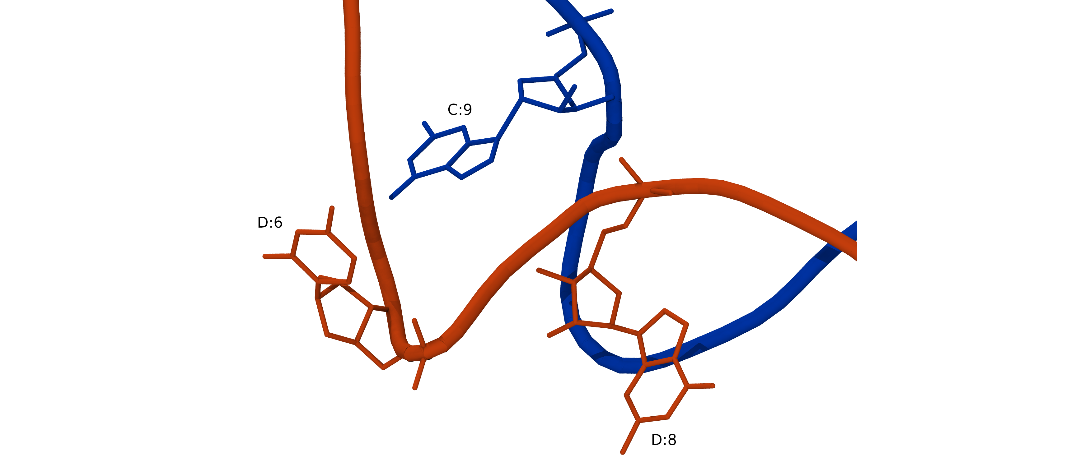
References
- SimRNA: a coarse-grained method for RNA folding simulations and 3D structure prediction
- SimRNA manual
- VMD TCL commands
4. Preparing simulation system for molecular dynamics.
4.1 Determine the number of water and salt molecules needed to prepare solvated system.
To prepare solution with the desired ionic strength we will use SLTCAP server. For this calculation we need to know the molecular weight of the macromolecules, their charge, and the number of water molecules in the simulation system.
The molecular weight of hAgo2 is 97,208 Da, and the MW of our nucleic acids is 12.5 KDa [calculate MW of the RNA]. Thus, the total MW is 110 KDa.
To determine the number of water molecules we will solvate the system in a cubic box extending 13 A from the solute.
mkdir -p ~/scratch/workshop/pdb/6N4O/simulation/setup
cd ~/scratch/workshop/pdb/6N4O/simulation/setup
cp ~/scratch/workshop/pdb/6N4O/protein_models/6n4o_chain_A_complete_A669D.pdb .
cp ~/scratch/workshop/pdb/6N4O/protein_models/4w5o_MG_ions.pdb .
cp ~/scratch/workshop/pdb/6N4O/RNA_models/simRNA/chains_CD_minimized.pdb .
Launch Leap and load protein and RNA forcefields:
module purge
module load gcc/9.3.0 cuda/11.4  ambertools/22
source $EBROOTAMBERTOOLS/amber.sh
tleap -f leaprc.RNA.OL3 -f leaprc.protein.ff14SB -f leaprc.water.tip3p -I $EBROOTAMBERTOOLS/dat/leap/lib/
Load pdb files into leap, combine them, and solvate the system
loadoff terminal_monophosphate.lib
rna = loadpdb chains_CD_minimized.pdb
prot = loadpdb 6n4o_chain_A_complete_A669D.pdb
mg = loadpdb 4w5o_MG_ions.pdb
sys = combine {prot,rna,mg}
solvatebox sys TIP3PBOX 13 iso
charge sys
quit
 Solute vdw bounding box:              110.734 72.027 85.780
  Total bounding box for atom centers:  136.734 136.734 136.734
      (box expansion for 'iso' is  70.6%)
  Solvent unit box:                     18.774 18.774 18.774
  Volume: 2740120.355 A^3
  Total mass 1460910.325 amu,  Density 0.885 g/cc
  Added 74991 residues.
> charge sys
Total unperturbed charge:  -6.000000
Total perturbed charge:    -6.000000
Using this information (MW 110 KDa, charge -6.0, 75000 water molecules) as an input to SLTCAP server we obtain the number of ions: 188 anions and 194 cations.
Determine protonation states of titratable sites in the model complex.
Use H++ server to determine what titratable sites in the model of protein-RNA complex 6n4o are in non-standard protonation state at pH 7?
Solution
For processing with H++ server we need to merge models of protein, nucleic acids and MG ions into one PDB file. As H++ server does not have library entries for phosphorylated 5’ terminals remove all 5’ phosphate atoms.
module purge
module load gcc/9.3.0 cuda/11.4  ambertools/22
mkdir -p ~/scratch/workshop/pdb/6N4O/simulation/setup/Hpp
cd ~/scratch/workshop/pdb/6N4O/simulation/setup/Hpp
tleap -I $EBROOTAMBERTOOLS/dat/leap/lib/
source leaprc.RNA.OL3 source leaprc.protein.ff14SB source leaprc.water.tip3p loadoff terminal_monophosphate.lib rna=loadpdb ../chains_CD_minimized.pdb remove rna rna.1@P remove rna rna.1@OP1 remove rna rna.1@OP2 remove rna rna.1@OP3 remove rna rna.1@HP3 remove rna rna.22@P remove rna rna.22@OP1 remove rna rna.22@OP2 remove rna rna.22@OP3 remove rna rna.22@HP3 prot=loadpdb ../6n4o_chain_A_complete_A669D.pdb mg=loadpdb ../4w5o_MG_ions.pdb sys=combine {prot rna mg} savepdb sys 6n4o_Hpp.pdb quitProcess 6n4o_Hpp.pdb with H++ server.
Uncheck ‘Correct orientation’ in the calculation setup.
When calculation completes download the list of computed pKs (0.15_80_10_pH6.5_6n4o_Hpp.pkout)Examine the pK_(1/2) column for HIS, ASP, GLU.
grep ^HI 0.15_80_10_pH6.5_6n4o_Hpp.pkout
grep ^AS 0.15_80_10_pH6.5_6n4o_Hpp.pkout
grep ^GL 0.15_80_10_pH6.5_6n4o_Hpp.pkout
Histidines 77, 766, 822, and 829 are protonated (HIP)
4.2 Preparing the complete simulation system
Finally, we have all pieces, and are ready to prepare the complete simulation system:
- The protein model, 6n4o_chain_A_complete_A669D.pdb
- The nucleic model, chains_CD_minimized.pdb
- Magnesium ions 4w5o_MG_ions.pdb
- We need to add 188 Na+ and 188 Cl- ions
- We need to protonate HIS 77, 766, 822, and 829
module purge
module load gcc/9.3.0 cuda/11.4  ambertools/22
cd ~/scratch/workshop/pdb/6N4O/simulation/setup
tleap -I $EBROOTAMBERTOOLS/dat/leap/lib/
source leaprc.RNA.OL3
source leaprc.protein.ff14SB
source leaprc.water.tip3p
loadamberparams frcmod.phos_nucleic14SB
loadoff terminal_monophosphate.lib
rna = loadpdb chains_CD_minimized.pdb
prot = loadpdb 6n4o_chain_A_complete_A669D.pdb
mg = loadpdb 4w5o_MG_ions.pdb
sys = combine {prot,rna,mg}
set {sys.77 sys.766 sys.822 sys.829} name "HIP"
addions sys Na+ 0
savepdb sys inpcrd_noWAT.pdb
solvatebox sys TIP3PBOX 13 iso
addionsrand sys Na+ 188 Cl- 188
saveamberparm sys prmtop.parm7 inpcrd.rst7
savepdb sys inpcrd.pdb
quit
mv inpcrd.pdb inpcrd.rst7 prmtop.parm7 ../
The force field modification frcmod.phos_nucleic14SB is needed for simulation stability. It modifies AMBER parm10 set for 5’ terminal phosphate in nucleic acids, The values are taken from frcmod.phosaa14SB
Write a shell script reproducing all system preparation steps
We can run all leap commands interactively, but it would be convenient to have a single shell script that could reproduce all system preparation step when executed. How can we do it?
Leap was designed to read commands from a file (-f option). It does not support input from STDIN, so we can not use pipeline to send commands to its input. This is inconvenient because we need two scripts to prepare a simulation: one with leap commands, and another with commands to run leap itself. Fortunately, shell is very flexible, and we can eliminate two-file workflow by using a special command allowing to use a variable instead of file as an input.
Inside of the script create a multi line variable containing all commands:
var=$(cat << EOF
...
...
EOF)
Then pass this variable to leap using the
<(echo "$var")command instead of filename. This command will allow leap to read the output of the commandecho "$var"instead of the input filename .Solution
#!/bin/bash
# FILE <<< prep_system.sh >>>
module purge
module load gcc/9.3.0 cuda/11.4  ambertools/22

inputData=$(cat << EOF
loadamberparams frcmod.phos_nucleic14SB
loadoff terminal_monophosphate.lib
rna = loadpdb chains_CD_minimized.pdb
prot = loadpdb 6n4o_chain_A_complete_A669D.pdb
mg = loadpdb 4w5o_MG_ions.pdb
sys = combine {prot,rna,mg}
set {sys.77 sys.766 sys.822 sys.829} name "HIP"
addions sys Na+ 0
solvatebox sys TIP3PBOX 13 iso
addionsrand sys Na+ 189 Cl- 189
saveamberparm sys prmtop.parm7 inpcrd.rst7
savepdb sys inpcrd.pdb
quit
EOF)

tleap -f leaprc.RNA.OL3 -f leaprc.protein.ff14SB -f leaprc.water.tip3p \
-I $EBROOTAMBERTOOLS/dat/leap/lib/ -f <(echo "$inputData")
Key Points
?
Hands-on 3B: Simulating a Complex RNA-protein System
Overview
Teaching: 30 min
Exercises: 5 minQuestions
How to simulate with AMBER?
Objectives
Running simulations with AMBER
1.1 Energy minimization.
Before simulating a system we need to relax it. Any atomic clashes must be resolved, and potential energy minimized to avoid unphysically large forces that can crash a simulation.
Let’s check our model for clashes.
cd ~/workshop/pdb/6N4O/simulation/setup/
source ~/env-biobb/bin/activate
check_structure -i inpcrd_noWAT.pdb checkall
...
8 Steric severe clashes detected
 LYS  124.CA  G    877.N2     0.747 A
 ARG  277.NE  U    878.P      0.845 A
 LYS  525.CE  C    888.N4     0.961 A
 THR  556.CA  A3   898.C4'    0.614 A
 PRO  557.C   A    897.N3     0.487 A
 GLN  558.N   A    897.C4     0.751 A
 THR  559.CA  A3   898.N3     0.435 A
 HIP  822.CD2 C    888.OP1    0.786 A
 ...
As the RNA model was built without protein, it is expected that the added RNA residues may be placed too close to some aminoacid residues. You can inspect severe clashes between the protein and the RNA residues visually to ensure that there are no severe problems that can not be fixed automatically (such as overlapping ring structures).
There is nothing too serious that may crash simulation, the clashes will be resolved in the process of energy minimization. As we want to keep our initial simulation structure as close to the experimental structure as possible we first allow energy minimizer to move freely only new added residues, and restrain all original residues. So we need a list of all original atoms to restrain them.
In the simulation system residues are renumbered. Chain identifiers are not used. There is a single list of all atoms where atoms and residues are numbered sequentially starting form 1 without any gaps. To make a list of restrained atoms we need to convert PDB residue numbers to simulation residue numbers. Residue number mapping between the original PDB file and the simulation is as follows:
| Chain | Original | Shift | Simulation |
|---|---|---|---|
| Protein A | 1-859 | - | 1-859 |
| RNA chain C | 1-21 | 859 | 860-880 |
| RNA chain D | 1-18 | 898 | 881-898 |
| MG ions | - | - | 899-901 |
Selecting atoms in a simulation system
- Create AMBERMASK representing all residues in the simulation system that are given in the original pdb entry 6N4O.
- Modify the AMBERMASK that you created to narrow selection to only backbone atoms.
Use the following definition of backbone atoms/: CA, N, O, P for protein, and P, C4’, O3’ for nucleic. Consult the AMBER mask selection manual.
Solution
- :22-120,126-185,190-246,251-272,276-295,303-819,838-858,860-868,870-877,879-885,889-896
- (:22-120,126-185,190-246,251-272,276-295,303-819,838-858,860-868,870-877,879-885,889-896)&(@CA,N,O,P,C4’,O3’)
The general minimization strategy is first to restrict all solute atoms with the experimental coordinates and relax all atoms that were added. (solvent, ions and missing fragments). This will help to stabilize the native conformation. There are no strict rules defining how many minimization steps are necessary. The choice will depend on the composition of a simulation system. For a big systems with a large amount of missing residues it is safer to carry out several minimization steps gradually releasing restraints. For example, you can first relax only solvent and ions, then lipid bilayer (if this is a membrane protein), then added fragments, then the original protein side-chains. Having more steps may be unnecessary, but it will not cause any problems.
Let’s do a two a two stage minimization. In the first stage we restrain all original atoms. In the second stage we restrain only the original backbone atoms.
cd ~/scratch/workshop/pdb/6N4O/simulation/sim_pmemd/1-minimization
Simulation programs can do a lot of different things, and every type of calculation has a number of parameters that allow us to control what will be done. To run a minimization we need to make an input file describing exactly what we want to do and how we want to do it:
- instruct a simulation program to minimize energy
- choose a method of minimization
- specify the maximum number of cycles of minimization
- apply restraints to a subset of atoms (optionally)
A simulation program reads simulation parameters from an input file. Simulation parameters in AMBER are called “FLAGS”. The Table below lists some important minimization FLAGS.
AMBER minimization parameters
| Flag | Value | Description |
|---|---|---|
| imin | 1 | Turn on minimization |
| ntmin | 0,1,2,3 | Flag for the method of minimization |
| maxcyc | integer | The maximum number of cycles of minimization |
| ncyc | integer | If NTMIN=1 switch from SD to CG after NCYC cycles |
| ntpr | integer n | Print energies every n steps |
| ntr | 1 | Use cartesian harmonic restraints |
| restraint_wt | float | Restraint force kcal/mol |
| restraintmask | ambermask | Specifies restrained atoms |
Methods of minimization
| 0 | Steepest descent+conjugate gradient. The first 4 cycles are steepest descent at the start of the run and after every non-bonded pair-list update. |
| 1 | For NCYC cycles the steepest descent method is used then conjugate gradient is switched on. |
| 2 | Steepest descent only |
| 3 | XMIN family methods. The default is LBFGS (Limited-memory Broyden-Fletcher-Goldfarb-Shanno). It is a popular algorithm in machine learning. The method incrementally learns from previous steps, so that it can make the next step more accurate. It converges considerably faster than CG, but requires more memory. |
Example minimization input file min_1.in
Title line. Energy minimization, stage 1.
&cntrl
imin=1, ntmin=0, maxcyc=200,    ! Minimization, method, number of cycles
ntpr=5,                         ! Print energies every ntpr steps
ntr=1,                          ! Use harmonic cartesian restraints
restraint_wt=100.0,             ! Restraint force kcal/mol
restraintmask="(:22-120,126-185,190-246,251-272,276-295,303-819,838-858,860-868,870-877,879-885,889-896)",
&end
END
Allocate resources. The workshop resources are limited, do not ask for more than 8 tasks.
salloc --time=2:0:0 --mem-per-cpu=2000 --ntasks=8
Load AMBER module and run minimization
module purge
module load gcc/9.3.0 cuda/11.4 ambertools/22
mpiexec sander.MPI -O -i min_1.in -p prmtop.parm7 -c inpcrd.rst7 -ref inpcrd.rst7 -r minimized_1.nc -o mdout_1&
The option -O means: overwrite the output files if present.
The output from the minimization goes into the file mdout. The total energy of the system is printed in the lines beginning with “EAMBER =”. If minimization is successful we expect to see large negative energies.
Why minimization fails?
When you run minimization with the input file min1.in as described above the program crashes after 4 cycles. Try to understand why minimization is unstable, and how to fix the problem.
Solution
With ntmin=0 the minimization method is switched from SD to CG only 4 SD cycles. As initial system has very high energy, 4 SD cycles are not sufficient to relax it well enough for CG to work.
Try to increase the number of CG cycles to 30 (ntmin=1, ncyc=30).
Examine mdout. How many SD steps are needed for total energy to become negative?
Try using an alternative minimization method (SD only or LBFGS). What method converges faster?
In the second round of minimization constrain only backbone atoms of all original residues. The mask for this selection will be
(:22-120,126-185,190-246,251-272,276-295,303-819,838-858,860-868,870-877,879-885,889-896)&(@CA,N,O,P,C4',O3')
Continue minimization from the restart coordinates:
mpiexec sander.MPI -O -i min_2.in -p prmtop.parm7 -c minimized_1.nc -ref inpcrd.rst7 -r minimized_2.nc -o mdout_2&
1.2 Heating
cd ~/scratch/workshop/pdb/6N4O/simulation/sim_pmemd/2-heating
Try in the allocated interactive shell:
mpiexec sander.MPI -O -i heat.in -p prmtop.parm7 -c minimized_2.nc -ref inpcrd.rst7 -r heated.nc -o mdout&
Submit to the queue to run simulation with GPU accelerated pmemd.cuda.
#SBATCH --mem-per-cpu=4000M
#SBATCH --time=3:00:00
#SBATCH --gres=gpu:v100:1
#SBATCH --partition=all_gpus
module load StdEnv/2020 gcc/8.4.0 cuda/10.2 openmpi/4.0.3 amber
pmemd.cuda -O -O -i heat.in -p prmtop.parm7 -c minimized_2.nc -ref inpcrd.rst7 -r heated.nc -o heating.log
GPU version runs less than 1 min.
| Flag | Value | Description |
|---|---|---|
| dt | 0.001 | Time step, ps. Default 0.001 |
| ntt | 1 | Constant temperature, using the Berendsen weak-coupling algorithm. |
| tempi | 150 | Initial temperature. The velocities are assigned from a Maxwellian distribution at TEMPI |
| temp0 | 300 | Reference temperature at which the system is to be kept |
| tautp | 1 | Time constant, in ps, for heat bath coupling, default is 1 ps. |
| ntp | 1 | Flag for constant pressure dynamics. 1 - MD with isotropic position scaling |
| barostat | 1 | Berendsen (default) |
| pres0 | 1 | Reference pressure, default 1 bar |
| taup | 4 | Pressure relaxation time (in ps), default 1 |
| ntwx | 1000 | Every ntwx steps, the coordinates will be written to the mdcrd file |
| ntpr | 100 | Print energies in the log every 100 steps, default 50 |
Plotting energy components.
Extract selected energy components from MD log and save in a table.
cpptraj << EOF
readdata heating.log
writedata energy.dat heating.log[Etot] heating.log[TEMP] heating.log[PRESS] heating.log[VOLUME] time 0.1
EOF
Read table into pandas dataframe and plot
import pandas as pd
import matplotlib.pyplot as plt

df = pd.read_table('energy.dat', delim_whitespace=True)
df.columns=["Time", "Etot", "Temp", "Press", "Volume"]

df.plot(subplots=True, x="Time", figsize=(6, 8))
plt.legend(loc='best')
plt.show()
1.3 Equilibration
Constrained equilibration
cd ~/scratch/workshop/pdb/6N4O/simulation/sim_pmemd/3-equilibration
- Turn on restart flag
- Shorten BerendsenPressureRelaxationTime to 1000
- Decrease restraint force to 10 kcal/mol
- Run for 2 ns
| Flag | Value | Description |
|---|---|---|
| ntx | 5 | Coordinates and velocities will be read from a restart file |
| irest | 1 | Restart simulations |
Unconstrained equilibration
- Switch to Landevin dynamics
- Run for 2 ns.
Download log file and examine energy.
Ready for production.
1.4 Production
cd ~/scratch/workshop/pdb/6N4O/simulation/sim_namd/4-production
Run for 10 ns
#!/bin/bash
#SBATCH --mem-per-cpu=4000M
#SBATCH --time=3:00:00
#SBATCH --gres=gpu:v100:1
#SBATCH --partition=all_gpus
module load StdEnv/2020 gcc/8.4.0 cuda/10.2 openmpi/4.0.3 amber

pmemd.cuda -O -O -i md.in -p prmtop.parm7 -c equilibrated_2.nc -r rest.nc -o md.log
Managing trajectories
You can remove everything not essential for processing for example water and ions. The following command will remove everything except residues from 1 to 901 and save every second frame in the file mdcrd_nowat.nc
cpptraj<<EOF
parm prmtop.parm7
trajin mdcrd.nc 1 last 2
strip !(:1-901)
trajout mdcrd_nowat.nc
parmstrip !(:1-901)
parmwrite out prmtop_nowat.parm7
run
EOF
2. Running simulations with NAMD
2.1 Energy minimization
There are only two minimization methods in NAMD, conjugate gradient and simple velocity quenching. All input and output related parameters are configured in input files. NAMD takes only one command line argument, the name of the input file.
NAMD reads constraints from a specially prepared pdb file describing constraint force for each atom in a system. Constraint forces can be given in x,y,z, occupancy or beta columns.
| Parameter | Value | Description |
|---|---|---|
| minimization | on | Perform conjugate gradient energy minimization |
| velocityQuenching | on | Perform energy minimization using a simple quenching scheme. |
| numsteps | integer | The number of minimization steps to be performed |
| constraints | on | Activate cartesian harmonic restraints |
| conskfile | path | PDB file containing force constant values |
| conskcol | X,Y,Z,O,B | Column of the PDB file to use for the position restraint force constant |
| consref | path | PDB file containing restraint reference positions |
cd ~/scratch/workshop/pdb/6N4O/simulation/sim_namd/1-minimization
As we did in the previous section, in the first round of minimization we restrain all original atoms. Let’s prepare PDB file with constraint forces in the occupancy field for this run. Such files can be prepared with VMD.
module load vmd
vmd
mol new prmtop.parm7
mol addfile inpcrd.rst7
set sel [atomselect top "all"]
$sel set occupancy 0.0
set sel [atomselect top "noh resid 22 to 120 126 to 185 190 to 246 251 to 272 276 to 295 303 to 819 838 to 858 860 to 868 870 to 877 879 to 885 889 to 896"]
$sel set occupancy 100.0
set sel [atomselect top "all"]
$sel writepdb constrain_all.pdb
quit
Minimization input file min_1.in. In addition to input, output, constraints, and general minimization parameters this file describes force field and PME calculations.
# Minimization, restrained backbone
# Input
parmfile       prmtop.parm7
ambercoor      inpcrd.rst7
# Output
outputname          minimized_1
numsteps 400
# Constraints
constraints on
conskFile constrain_all.pdb
conskcol O
consref constrain_all.pdb
# Integrator
minimization   on
# AMBER FF settings
amber on
cutoff         9.0
pairlistdist   11.0
switching      off
exclude        scaled1-4
readexclusions yes
1-4scaling     0.83333333
scnb           2.0
ljcorrection   on
# PME
PME                 on
PMEGridSizeX        140
PMEGridSizeY        140
PMEGridSizeZ        140
# Periodic cell
cellBasisVector1   137  0.0 0.0
cellBasisVector2   0.0 137  0.0
cellBasisVector3   0.0 0.0  137
Run 500 steps of energy minimization:
module load StdEnv/2020 intel/2020.1.217 namd-multicore/2.14
charmrun ++local +p 8 namd2 min_1.in >&log&
In the second round of minimization constrain only backbone atoms of all original residues.
Prepare force constants file:
mol new prmtop.parm7
mol addfile inpcrd.rst7
set sel [atomselect top "all"]
$sel set occupancy 0.0
set sel [atomselect top "name CA N O P C4' O3' and resid 22 to 120 126 to 185 190 to 246 251 to 272 276 to 295 303 to 819 838 to 858 860 to 868 870 to 877 879 to 885 889 to 896"]
$sel set occupancy 10.0
set sel [atomselect top "all"]
$sel writepdb constrain_all_backbone_f10.pdb
quit
Run 1000 minimization steps.
charmrun ++local +p 8 namd2 min_2.in >&log&
2.2 Heating
After energy minimization we have the optimized coordinates that are ready for MD simulation.
cd ~/scratch/workshop/pdb/6N4O/simulation/sim_namd/2-heating
| Parameter | Value | Description |
|---|---|---|
| temperature | 150 | Generate velocities at 150 K |
| tCouple | on | Use Berendsen thermostat |
| tCoupleTemp | 300 | Temperatute of the heat bath |
| BerendsenPressure | on | Use Berendsen barostat |
| BerendsenPressureRelaxationTime | 4000 | Use long relaxation time to slow down box rescaling |
| numsteps | 20000 | The number of simulation steps |
2.3. Equilibration
Constrained equilibration
cd ~/scratch/workshop/pdb/6N4O/simulation/sim_namd/3-equilibration
Read velocities and box from the restart files
Shorten BerendsenPressureRelaxationTime to 1000
Run for 2 ns.
Unconstrained equilibration
Switch to Landevin dynamics
Run for 2 ns.
2.4 Production
cd ~/scratch/workshop/pdb/6N4O/simulation/sim_namd/4-production
Run for 10 ns.
3. Transferring equilibrated system between simulation packages.
Simulation packages have different methods and performance. It is useful to be able to transfer a running simulation from one software to another. Imagine that you started your project with GROMACS, but later realized that you need to run a constant pH simulation. You need to switch to AMBER. Want to study conformational transitions? Gaussian accelerated MD is not available in GROMACS. Another reason to move to AMBER/NAMD. Want to apply custom forces - move to NAMD.
3.1. Moving simulation from NAMD to AMBER.
NAMD saves coordinates, velocity and periodic box in separate files. In AMBER all information required to restart simulation is in one text (.rst7) or netcdf (.ncrst) file. To prepare AMBER restart file we first convert namd binary files to amber text restart files with VMD:
cd ~/scratch/Ago-RNA_sim/sim_pmemd/2-production
cp ~/scratch/Ago-RNA_sim/sim_namd/5-equilibration-unconstrained/{equilibration.coor,equilibration.vel,equilibration.xsc} .
module load intel vmd
vmd
# Convert velocities
mol new equilibration.vel type namdbin
set sel [atomselect top all]
$sel writerst7 vel.rst7
# Convert coordinates
mol new equilibration.coor
set sel [atomselect top "all"]
$sel writerst7 coor.rst7
quit
Now we can read these files along with the extended system (.xsc) file and prepare the complete rst7 file. We will do it with ParmEd, the program for editing AMBER parameter and coordinate files.
NAMD controls pressure differently from AMBER, so when we transfer simulation to AMBER pressure will be too high. It will relax on its own, but we can slightly rescale coordinates and periodic box to speed up pressure equilibration.
module purge
module load StdEnv/2020 gcc ambertools python scipy-stack
source $EBROOTAMBERTOOLS/amber.sh
python
import parmed as pmd
import numpy as np

sc=1.002
xsc = np.loadtxt('equilibration.xsc')
vel_rst7 = pmd.load_file('vel.rst7')
coor_rst7 = pmd.load_file('coor.rst7')
new_rst7 = pmd.amber.Rst7(natom=vel_rst7.natom)
new_rst7.vels = vel_rst7.coordinates*20.455
new_rst7.coordinates = coor_rst7.coordinates*sc
new_rst7.box = [xsc[1]*sc, xsc[5]*sc, xsc[9]*sc, 90, 90, 90]
new_rst7.title = "Created with ParmEd"
new_rst7.write("restart.rst7")
quit()
We converted NAMD restart files to AMBER restart and we can continue simulation with AMBER. AMBER suite includes several simulation codes: sander, sander.MPI, pmemd, pmemd.MPI, pmemd.cuda. Sander is free version, pmemd is commercial. Sander and pmemd are serial (CPU only) programs; sander.MPI and pmemd.MPI are parallel (CPU only); and pmemd.cuda is GPU version.
Submitting pmemd.cuda on Siku:
#SBATCH --mem-per-cpu=4000M
#SBATCH --time=3:00:00
#SBATCH --gres=gpu:v100:1
module load StdEnv/2020 gcc/9.3.0 cuda/11.4 openmpi/4.0.3 amber/20.12-20.15

pmemd.cuda -O -i pmemd_prod.in -o production.log -p ../../prmtop.parm7 -c restart.rst7
PMEMD is highly optimized to do all computations in one GPU, and it runs exceptionally fast. It CANNOT be used efficiently on more than one GPU because of the overhead from moving data between GPUs.
References: Amber file formats
3.2 Moving simulation from AMBER to GROMACS.
To transfer simulation to GROMACS in addition to converting restart file we need to convert topology.
First convert AMBER topology to GROMACS
module purge
module load StdEnv/2020 gcc/9.3.0 cuda/11.4 openmpi/4.0.3 ambertools/22
cd ~/scratch/workshop/pdb/6N4O/simulation/sim_gromacs/0-setup
python
import parmed as pmd
amber = pmd.load_file("prmtop.parm7", "inpcrd.rst7")
amber.save('topol.top')
amber.save('inpcrd.gro')
Make index files with groups of atoms that we want to restrain, (one for the original residues and another for backbone of the original residues).
To recap, the original residues are
:22-120,126-185,190-246,251-272,276-295,303-819,838-858,860-868,870-877,879-885,889-896
Position restraints are defined within molecule blocks, they must be included within the correct moleculetype block after all atoms are defined (after the atoms block). The end of the moleculetype block is a good place.
The atom numbers in position restraints .itp files must match the atom numbers in a corresponding moleculetype block. Our topology file gromacs.top includes several molecules. The protein is the first, system1 molecule. The nucleic acids are is the second system2 and the third system3 molecules.
WARNING: the genrestr program can generate the correct restraints file only for the first molecule. If you need to restrain the second molecule this tool will not work. To generate a valid constraint file you need to shift indexes in the posre.itp file by the number of atoms in the preceding molecule(s). This can be done by generating separate topology files for each of the RNA chains.
This is a long job, so for now we will restrain only protein. Let’s prepare position restraint files for system1.
gmx make_ndx -f inpcrd.gro <<EOF
del5-36
del6-7
r22-120|r126-185|r190-246|r251-272|r276-295|r303-819|r838-858
name 6 Orig_prot
6&aCA
6&aN
6&aO
7|8|9
del 7-9
name 7 Orig_prot_backbone
q
EOF
Check groups:
gmx make_ndx -n index.ndx
Generate positional restraints files, one for all original protein atoms, another for the backbone of the original protein residues.
gmx genrestr -f inpcrd.gro -fc 500.0 -n index.ndx -o orig_prot.itp<<EOF
Orig_prot
EOF
gmx genrestr -f inpcrd.gro -fc 50.0 -n index.ndx -o orig_prot_backbone.itp<<EOF
Orig_prot_backbone
EOF
Add definitions of the position restraints to the topology “gromacs.top”. Use a text editor of your choice to insert the following lines at the end of the system1 molecule block:
#ifdef ORIG_PROT_POSRES
#include "orig_prot.itp"
#endif
#ifdef ORIG_PROT_BACKBONE
#include "orig_prot_backbone.itp"
#endif
Now we can include any of these two files from the minimization input file by defining a corresponding variable
; Turn on position restraints
define = -DORIG_PROT_POSRES
; Run parameters
integrator              = steep
nsteps                  = 400
; Output control
nstxout                 = 0
nstvout                 = 0
nstfout                 = 0
nstenergy               = 5
nstlog                  = 5
nstxout-compressed      = 2000
; Bond parameters
continuation            = no
constraint_algorithm    = shake
constraints             = h-bonds
; Neighbor-searching
cutoff-scheme           = Verlet
nstlist                 = 10
rcoulomb                = 0.8
rvdw                    = 0.8
DispCorr                = Ener ; anaytic VDW correction
; Electrostatics
coulombtype             = PME
pme_order               = 4
fourier-nx              = 140
fourier-ny              = 140
fourier-nz              = 140
Make binary topology
gmx grompp -f min.mdp -p gromacs.top -c inpcrd.gro -r inpcrd.gro -o input.tpr<<EOF
q
EOF
import parmed as pmd
amber = pmd.load_file('../prmtop.parm7', '../sim_pmemd/2-production/restart.rst7')
amber.save('gromacs.top')
Then convert velocities and coordinates:
Amber operates in kcal/mol units for energy, amu for masses, and Angstoms for distances. For convenience when calculating KE from velocity, the velocities have a conversion factor built in; as a result the Amber unit of time is (1/20.455) ps. So to convert Amber velocities from internal units to Ang/ps multiply by 20.455. The number itself is derived from sqrt(1 / ((AMU_TO_KG * NA) / (1000 * CAL_TO_J))).
vel_rst7 = pmd.load_file('../sim_pmemd/2-production/vel.rst7')
amber.velocities = vel_rst7.coordinates*20.455
amber.save('restart.gro')
module load StdEnv/2020 gcc/9.3.0 openmpi/4.0.3 gromacs
gmx trjconv -f restart.gro -o restart.trr
gmx make_ndx -f restart.gro
gmx grompp -p gromacs.top  -c restart.gro -t restart.trr -f gromacs_production.mdp
Running simulation
#SBATCH --mem-per-cpu=4000M
#SBATCH --time=10:00:00
#SBATCH --cpus-per-task=16
module load StdEnv/2020 gcc/9.3.0 openmpi/4.0.3 gromacs
gmx mdrun -s input.tpr
Key Points
Hands-on 4: Preparing a system for simulation with GROMACS
Overview
Teaching: 30 min
Exercises: 5 minQuestions
How to Prepare Input Files for Simulation with GROMACS?
Objectives
Learn to Generate Input Files for Simulation with GROMACS
Generating Input Files for Simulation with GROMACS.
What force fields are available in the loaded GROMACS module?
When the GROMACS module is loaded the environment variable EBROOTGROMACS will be set. This variable is pointing to the GROMACS installation directory. Knowing where the GROMACS installation is we can find out what force fields are available:
module load gromacs
ls -d $EBROOTGROMACS/share/gromacs/top/*.ff | xargs -n1 basename
amber03.ff amber99sb-ildn.ff gromos45a3.ff amber94.ff amberGS.ff gromos53a5.ff amber96.ff charmm27.ff gromos53a6.ff amber99.ff gromos43a1.ff gromos54a7.ff amber99sb.ff gromos43a2.ff oplsaa.ff
Generate GROMACS Topology and Coordinate Files from the Solvated System.
cd ~/scratch/workshop/pdb/1RGG/GROMACS
We can generate GROMACS topology from the complete simulation system prepared previously and saved in the file 1RGG_chain_A_solvated.pdb. For pdb2gmx to work correctly we need to rename ions from (Na+, Cl-) to (NA, CL), and rename CYX to CYS:
ATOM   1444 Na+  Na+    97      -5.058 -11.031  -0.206  1.00  0.00
ATOM   1450 Cl-  Cl-   103      19.451  -3.022   8.361  1.00  0.00
We will also assign ions to chain B.
mol new ../1RGG_chain_A_solvated.pdb
set s [atomselect top "resname 'Na+'"]
$s set resname "NA"
$s set name "NA"
$s set chain "B"
set s [atomselect top "resname 'Cl-'"]
$s set resname "CL"
$s set name "CL"
$s set chain "B"
set s [atomselect top "resname CYX"]
$s set resname "CYS"
set s [atomselect top all]
$s writepdb 1RGG_chain_A_solvated_gro.pdb
quit
- Do it using the global substitution function of the stream editor (sed).
cat ../1RGG_chain_A_solvated.pdb |\
sed s/"Cl-  Cl-  "/" CL  CL  B"/g |\
sed s/"Na+  Na+  "/" NA  NA  B"/g |\
sed s/CYX/CYS/g > 1RGG_chain_A_solvated_gro.pdb
Let’s make the topology using the AMBER ff99SBildn force field and the tip3 water model:
gmx pdb2gmx -f 1RGG_chain_A_solvated_gro.pdb -ff amber99sb-ildn -water tip3 -ignh -chainsep id -ss << EOF
y
EOF
| Option | Value | Description |
|---|---|---|
| ignh | - | Ignore hydrogens in file |
| chainsep | id | Separate chains by chain ID. Since we assigned ions to chain B pbb2gmx will ignore TER records and put them in a separate chain |
| ss | - | Interactive S-S bridge selection. Detect potential S-S bonds, and ask for confirmation. |
The construct
<< EOF
y
EOF
at the end of the command is to automatically confirm ‘y’ S-S bond.
By default pdb2gmx program saved three output files:
| Type | Filename |
|---|---|
| topology | topol.top |
| coordinates | conf.gro |
| position restraints | posre.itp |
The names of the output files can be changed by using output options -p, -o and -i.
Prepare the System Using GROMACS Module pdb2gmx.
To demonstrate how to solvate protein and add ions using pdb2gmx we can go back to the protein structure file 1RGG_chain_A_prot.pdb saved before solvation and repeat all system preparation steps with this GROMACS utility. Note that in this case the neutralizing ions will be added in randomly selected positions.
First we generate the topology and the coordinate file using the AMBER ff99SBildn force field and the spc/e water model:
gmx pdb2gmx -f ../1RGG_chain_A_prot.pdb -ff amber99sb-ildn -water tip3 -ignh -chainsep id -ss << EOF
y
EOF
Once the gromacs coordinate file conf.gro is created we add a periodic box to it:
gmx editconf -f conf.gro -o boxed.gro -c -d 1.5 -bt cubic
The option ‘-c’ positions solute in the middle of the box, the option -d specifies the distance (in nm) between the solute and the box. Add water
gmx solvate -cp boxed.gro -cs spc216.gro -o solvated.gro -p topol.top
Next, we need to create a binary topology file. For this we need a MD run parameters file. An empy file will be sufficient for now. Using the empty file ‘mdrun.mdp’ we can generate the binary topology ‘solvated.tpr’ file:
touch mdrun.mdp
gmx grompp -f mdrun.mdp -p topol.top -c solvated.gro -o solvated.tpr >& grompp.log
When the grompp program runs it generates a lot of diagnostic messages and prints out the net charge. We saved the output in the file ‘grompp.log’ so that we can find out what is the total charge of the system:
grep "total charge" grompp.log
System has non-zero total charge: -5.000000
Finally we can use the GROMACS genion command to replace random solvent molecules with ions. We will first add cation/anion pairs to mimic a desired salt concentration and then neutralize the system by adding sodium ions (the options -conc [Mol/L] and -neutral). By default genion uses Na+ and Cl- ions. Other ions can be chosen by selecting options -pname [positive ion] and -nname [negative ion]. We also need to select a target group of solvent molecules to be replaced with ions. We will chose the ‘SOL’ group which is the default name of the solvent group in GROMACS:
$ echo "SOL" | gmx genion -s solvated.tpr -p topol.top -neutral -conc 0.15 -o neutralized.pdb
Let’s inspect the last section of the updated topology file:
tail -n 4 topol.top
Protein_chain_A     1
SOL         11482
NA               38
CL               33
Create a binary topology file with the new topology and run parameters.
gmx grompp -f minimization.mdp -p topol.top -c neutralized.pdb -o solvated_neutral.tpr
You can see that 38 sodium and 33 chloride ions were added to the system.
Why PDB to GROMACS conversion fails?
Download the structure file 2F4K from PDB and try to generate the molecular topology with pdb2gmx:
wget http://files.rcsb.org/view/2F4K.pdb
gmx pdb2gmx -f 2F4K.pdb -ff amber99sb-ildn -water spce
Why this command fails and how to fix it?
Solution
The file contains two noncanonical norleucine aminoacids (NLE65 and 70). GROMACS does not have parameters for this aminoacid. You have two options: replace norleucine with leucine or add norleucine parameters.
Key Points
Hands-on 5: Generating topologies and parameters for small molecules.
Overview
Teaching: 30 min
Exercises: 5 minQuestions
How to parameterize small molecules?
Objectives
Parameterize hexanediol
Generating topologies and parameters for small molecules.
ANTECHAMBER
Download hexanediol 3D structure
- Find hexanediol (compound 147023) in PubChem and download 3D SDF file.
- Convert SDF to PDB using Open Babel and change residue name:
cd ~/workshop_amber/example_05
module purge
module load StdEnv/2023 openbabel
obabel Conformer3D_COMPOUND_CID_147023.sdf -O hexanediol.pdb
sed  "s/UNL/HEZ/g" hexanediol.pdb > HEZ.pdb
Make mol2 file with antechamber
module purge
module load StdEnv/2023 ambertools/23
antechamber -i HEZ.pdb -fi pdb -o HEZ.mol2 -fo mol2 -c bcc -s 2
The file HEZ.mol2 contains the definition of our HEZ residue including connectivity, all of the charges and atom types.
Run parmchk2 to find out if there are any missing force field parameters
parmchk2 -i HEZ.mol2 -f mol2 -o HEZ.frcmod
If it can antechamber will fill in these missing parameters by analogy to a similar parameter.
Create the library file for HEZ using tleap:
source leaprc.gaff2
HEZ=loadmol2 HEZ.mol2
check HEZ
saveoff HEZ hez.lib
Of course point charges are not very accurate because they are derived using semi-empirical method, but antechamber can also use results of gaussian QM calculations.
Deriving accurate point charges
User can derive charges using RESP and supply them in mol2 file.
Electrostatic Parameterization with py_resp.py
- QM Geometry Optimization (gaussian)
- Electrostatic Potential Calculation (gaussian)
- Convert the Gaussian ESP data format for PyRESP (ambertools:espgen)
- Generate input for py_resp.py (ambertools:pyresp_gen.py)
- RESP Parameterization (ambertools:py_resp.py)
Charge derivation methods
Activity 1: Derive RESP, CM5 and AM1-BCC2 (sqm) charges and compare them
Activity 2: Compare binding free energy calculated using different charge sets.
Comparison of Charge Derivation Methods Applied to Amino Acid Parameterization. - Derivation does not matter much for aminoacids?
Molecular Insights into the Covalent Binding of Zoxamide to the β-Tubulin of Botrytis cinerea - Some ligands for exercise on parameterization: carbendazim (CBZ), diethofencarb (DEF), zoxamide (ZOX)
- Retrieve from Pubmed, Optimize using QUICK (B3LYP/6-31G*)
AnteChamber PYthon Parser interfacE (ACPYPE)
ANTECHAMBER, a module of the AmberTools package, is the main tool for creating topological parameters in AMBER force fields. It can be used to generate topologies for most organic molecules.
ACPYPE - AnteChamber PYthon Parser interfacE.
- Simplifies and automates generation of topology and parameters in different formats for different molecular mechanics programs.
- Translates force field to GROMACS
Installing and using ACPYPE on the Aliiance clusters
module load  python  openbabel
virtualenv ~/venv_acpype
source ~/venv_acpype/bin/activate
pip install --no-index acpype
Create force field files:
acpype -i HEZ.pdb -n 0
Free energy calculations
MMPBSA
Prepare tolopogies:
ante-MMPBSA.py -p ../../start.prmtop -s '!(:214-456,669-1029)' -c complex.prmtop
ante-MMPBSA.py -p complex.prmtop -n ':1-243' -l ligand.prmtop -r receptor.prmtop
-s Amber mask of atoms needed to be stripped from PRMTOP to make the COMPLEX topology file
-n Amber mask of atoms needed to be stripped from COMPLEX to create LIGAND.
Input file for running PB and GB in serial
&general
   startframe=0, endframe=10, interval=1,
   keep_files=2, verbose=1, use_sander=1,
   strip_mask=!(:214-456,669-1029),
   ligand_mask=:1-243, receptor_mask=:244-604,
/
&gb
  igb=2, saltcon=0.150,
/
#!/bin/bash
#SBATCH --ntasks=10
#SBATCH --mem-per-cpu=4000M
#SBATCH --time=3:00:00
module purge
module load StdEnv/2020 gcc/9.3.0 openmpi/4.0.3 ambertools/23
MMPBSA.py.MPI -O -i mmpbsa.in -o FINAL_RESULTS_MMPBSA.dat -sp ../../start.prmtop -cp complex.prmtop -rp receptor.prmtop -lp ligand.prmtop -y ../../../min/min.dcd
Memory requirements
Generalized Born: 3N (atom positions) + 2N (atom parameters) + data structures for evaluating the full energy. GB memory requirements should scale more or less linearly with the number of atoms in the system
Normal modes: slightly more than (3N * 3N)/2 to store Hessian matrix + data structures for evaluating the full energy. The major expense here is the N^2 scaling of the Hessian storage.
Poisson Boltzmann: the memory is dominated primarily by the grid, it depends strongly on the grid spacing.
3D-RISM: also requires a grid. The 3D-RISM grid needs to be denser than the corresponding grid for PB, so RAM requirements for 3D-RISM are typically a bit higher than PB.
Key Points
Hands-on 6: A Comparative Performance Ranking of the Molecular Dynamics Software
Overview
Teaching: 30 min
Exercises: 5 minQuestions
How to evaluate CPU efficiency of a simulation?
How fast and efficient my simulation will run with different programs and computing resources?
Objectives
Learn how to request the right computational resources
Requesting the right computational resources is essential for fast and efficient simulations. Submitting a simulation with more CPUs does not necessarily mean that it will run faster. In some cases, a simulation will run slower with more CPUs. There is also a choice between using CPU or GPU versions. When deciding on the number of CPUs, it is crucial to consider both simulation speed and CPU efficiency. If CPU efficiency is low, you will be wasting resources. This will negatively impact your priority, and as a result, you will not be able to run as many jobs as you would if you used CPUs more efficiently. To assess CPU efficiency, you need to know how fast a serial simulation runs and then compare the expected 100% efficient speedup (speed on 1CPU x N) with the actual speedup on N CPUs.
Here is the chart of the maximum simulation speed of all MD engines tested on the Alliance systems. These results may give you valuable insight into how fast and efficient you can expect your simulation to run with different packages/resources.
Submission scripts for running the benchmarks.
GROMACS
Extend simulation for 10000 steps
gmx convert-tpr -s topol.tpr -nsteps 10000 -o next.tpr
Submission script for a CPU simulation
#SBATCH --mem-per-cpu=4000M
#SBATCH --time=10:00:00
#SBATCH --ntasks=2
#SBATCH --cpus-per-task=4

module load StdEnv/2020 gcc/9.3.0 openmpi/4.0.3 gromacs/2023.2
export OMP_NUM_THREADS="${SLURM_CPUS_PER_TASK:-1}"

srun gmx mdrun -s next.tpr -cpi state.cpt
Submission script for a single GPU simulation
#!/bin/bash
#SBATCH --mem-per-cpu=2000M
#SBATCH --time=1:00:00
#SBATCH --cpus-per-task=12
#SBATCH --gpus-per-node=1

module load StdEnv/2020 gcc/9.3.0 cuda/11.4 openmpi/4.0.3 gromacs/2023.2

gmx mdrun -ntomp ${SLURM_CPUS_PER_TASK:-1} \
    -nb gpu -pme gpu -update gpu -bonded cpu -s topol.tpr
Submission script for a multiple GPU simulation
#!/bin/bash
#SBATCH --mem-per-cpu=2000M
#SBATCH --time=1:00:00
#SBATCH --nodes=1
#SBATCH --ntasks-per-node=2
#SBATCH --cpus-per-task=12
#SBATCH --gpus-per-task=1

module load StdEnv/2020 gcc/9.3.0 cuda/11.4 openmpi/4.0.3 gromacs/2023.2

srun gmx mdrun -ntomp ${SLURM_CPUS_PER_TASK:-1} \
-nb gpu -pme gpu -update gpu -bonded cpu -s topol.tpr
PMEMD
Submission script for a single GPU simulation
#!/bin/bash
#SBATCH --cpus-per-task=1
#SBATCH --gpus 1
#SBATCH --mem-per-cpu=2000M
#SBATCH --time=1:00:00

module --force purge
module load StdEnv/2020  gcc/9.3.0 cuda/11.4 openmpi/4.0.3 amber/20.12-20.15
pmemd.cuda -O -i pmemd.in -o production.log -p prmtop.parm7 -c restart.rst7
Submission script for a multiple GPU simulation
Multiple GPU pmemd version is meant to be used only for AMBER methods running multiple simulations, such as replica exchange. A single simulation does not scale beyond 1 GPU.
#!/bin/bash
#SBATCH --nodes=1
#SBATCH --ntasks-per-node=2
#SBATCH --gpus-per-node=2
#SBATCH --mem-per-cpu=2000M
#SBATCH --time=1:00:00

module --force purge
module load StdEnv/2020  gcc/9.3.0 cuda/11.4 openmpi/4.0.3 amber/20.12-20.15

srun pmemd.cuda.MPI -O -i pmemd_prod.in -o production.log \
        -p prmtop.parm7 -c restart.rst7
NAMD 3
Submission script for a GPU simulation
#!/bin/bash
#SBATCH --cpus-per-task=2
#SBATCH --gpus-per-node=a100:2
#SBATCH --mem-per-cpu=2000M
#SBATCH --time=1:00:00
NAMDHOME=$HOME/NAMD_3.0b3_Linux-x86_64-multicore-CUDA

$NAMDHOME/namd3 +p${SLURM_CPUS_PER_TASK} +idlepoll namd3_input.in
How to make your simulation run faster?
It is possible to increase time step to 4 fs with hydrogen mass re-partitioning. The idea is that hydrogen masses are increased and at the same time masses of the atoms to which these hydrogens are bonded are decreased to keep the total mass constant. Hydrogen masses can be automatically re-partitioned with the parmed program.
module --force purge
module load StdEnv/2020 gcc ambertools python scipy-stack
source $EBROOTAMBERTOOLS/amber.sh
parmed prmtop.parm7
ParmEd: a Parameter file Editor

Loaded Amber topology file prmtop.parm7
Reading input from STDIN...
> hmassrepartition
> outparm prmtop_hmass.parm7
> quit
References:
1.Lessons learned from comparing molecular dynamics engines on the SAMPL5 dataset
2.Delivering up to 9X the Throughput with NAMD v3 and NVIDIA A100 GPU
3.AMBER GPU Docs
4.Long-Time-Step Molecular Dynamics through Hydrogen Mass Repartitioning
Key Points
To assess CPU efficiency, you need to know how fast a serial simulation runs