Using VMD on Digital Research Alliance of Canada systems
Overview
Teaching: 10 min
Exercises: 5 minQuestions
What is VMD used for?
How to use VMD remotely on Alliance clusters?
Objectives
Learn how to run vmd on a compute node
Learn how to connect graphically to VMD running on a compute node
Introduction
Molecular modelling and simulations are widely used in structural biology, chemistry, drug design, materials science and many other fields of science. Visualization is one of the most useful means for evaluating the quality of molecular models. The ability to visualize atomic details is crucial to understanding molecular functions.
Visualizing macromolecular structures is challenging, and it requires specialized software. VMD is one of the molecular visualization packages. Alternative molecular visualization software includes UCSF Chimera, PyMol, and JMol
VMD (Visual Molecular Dynamics) is a software package for the 3D visualization, modeling and analysis of molecular systems. It is developed and freely distributed by the Theoretical and Computational Biophysics Group at the University of Illinois at Urbana-Champaign.
- VMD (Visual Molecular Dynamics) is a software package for the 3D visualization, modeling and analysis of molecular systems.
VMD features
- VMD works efficiently with large trajectories.
- VMD supports
- wide variety of file formats
- photorealistic rendering of images
- VMD offers
- built-in tools and plugins for analysis of structures and trajectories
- powerful scripting capability
- ability to make custom trajectory movies
Using VMD on a remote server
The trajectory files generated by MD simulations are large, so transferring them to your local computer can be time-consuming. By visualizing and analyzing them remotely, you could save a lot of time and efforts. That’s why, we’ll start our workshop by showing you how to use VMD remotely. I encourage you to consider remote connection, but if you are not comfortable with this you can use your own computer.
To use VMD GUI on Alliance clusters you need to establish graphical connection. Currently there are two options: remote desktop with VNC or JupyterHub.
- To use VMD GUI on Alliance clusters you need to establish graphical connection.
- There are two options: remote desktop with VNC or JupyterHub.
Connecting to the training cluster
- ssh: moledyn.ace-net.training
- JupyterHub: jupyter.moledyn.ace-net.training
- Login sheet
Connecting graphically to a cluster with JupyterHub
JupyterHub provides remote desktop via noVNC (the open source VNC client). JupyterHub runs in any browser. It is convenient to use as it allocates resources and launches remote desktop in one step without requiring any additional software.
Here is the list of JupyterHubs on clusters.
Steps to connect to a Jupyter Hub:
- Login with your CC credentials
- Request resources and spin up a Jupyter server
- Choose
Desktopin JupyterLab Launcher
The drawbacks:
- If cluster usage is high the Jupyter server may fail to start due to a timeout.
- Does not support copy/paste from the host machine
Connecting graphically to a cluster using TigerVNC
Connecting to a visualization node on Graham
Graham has dedicated visualization nodes. You need to install TigerVNC Viewer to use them (RealVNC or any other client will not work). To start using a dedicated visualization node simply connect TigerVNC viewer to gra-vdi.alliancecan.ca.
Advantages:
- Direct and simple connection from your laptop with TigerVNC Viewer.
- Offer Nvidia GPUs for hardware-accelerated rendering of images
Drawbacks:
- Available only on Graham
No modules are loaded on VDI nodes by default. Before you can use central modules you need to load CcEnv and StdEnv modules:
module load CcEnv StdEnv/2023 vmd
If graphical window is off screen, you can reposition and resize it. The following commands should work for most of you:
display reposition 400 400
display resize 600 600
You can save your settings in the VMD initialization file. I’ll show you how to do it later.
Connecting graphically to a compute node (more challenging)
The VNC connection to a compute node is a little more complicated, but it is reliable. In addition, you’ll be able to copy/paste text into a remote desktop with VNC.
We will use Beluga as an example to illustrate connecting VNC to a compute node.
1. Connect to Beluga with SSH.
ssh user@beluga.computecanada.ca
2. Allocate some resources:
salloc -c2 --mem-per-cpu=1000 --time=3:0:0
...
salloc: Granted job allocation 35464975
salloc: Waiting for resource configuration
salloc: Nodes bg11308 are ready for job
[user@bg11308 ~]$
3. Start VNC server
vncserver
Enter your new VNC password when prompted. Answer ‘no’ on the question about view-only password.
Server will display a line like this in its output after it has started:
New 'bg11308.int.ets1.calculquebec.ca:1 (user)' desktop is bg11308.int.ets1.calculquebec.ca:1
Here bg11308 is the hostname of the node where the server is running and :1 is the number of VNC session.
TigerVNC sessions are listening on port 5900 plus the session number, so in this example port number is 5900 + 1 = 5901. You will need host name and port number to connect your computer to the remote VNC session.
4. Open SSH tunnel to the remote computer
Now you need to connect your local computer to the node where the VNC server is listening. In order to access compute nodes, you must go through a login node as they are located on an internal network.
We can use SSH client program to connect port 5901 of bg11308 directly to our local computer. This type of connection is called “SSH tunneling” or “SSH port forwarding”.
The following SSH command creates a tunnel between port 5901 on bg11308 and port 5901 on your local computer.
ssh user@beluga.computecanada.ca -L 5901:bg11308:5901
The format of the host:port specification is local_port:remote_host:remote_port. You can use any free local port.
The tunnel is active only while the session is running. Do not close this window and do not logout, this will close the tunnel and disconnect your laptop.
5. Connect the local computer to the remote computer
Start VNC viewer on your local computer and connect it to localhost:5901.
6. When you are done close VNC session on the remote:
vncserver -kill :1
If you don’t terminate VNC sessions old .log and .pid files will be accumulating in the directory ~/.vnc, but don’t worry, it is easy to clean them up:
rm ~/.vnc/*.log
rm ~/.vnc/*.pid
Challenge
What ssh command should user21 use to connect port 5999 of his laptop to VNC session :5 running on node2 of the cluster moledyn.ace-net.training?
Answers:
- ssh user21@moledyn.ace-net.training -L 5999:localhost:5905
- ssh user21@moledyn.ace-net.training -L 5905:localhost:5999
- ssh user21@moledyn.ace-net.training -L 5999:node2:5905
- ssh user21@node2.ace-net.training -L 5999:localhost:5905
Solution
ssh user21@moledyn.ace-net.training -L 5999:node2:5905
Key Points
Connect to a compute node using TigerVNC client and SSH tunnel
Loading Structure Files and Interacting with Molecules
Overview
Teaching: 30 min
Exercises: 10 minQuestions
How to load PDB files into VMD?
How to view molecules interactively?
How to measure distances, angles and dihedrals?
Objectives
Learn how to load molecular structure files
Learn how to interact with molecules
Learn how get information about atoms and molecules
Learn how to measure distances, angles and dihedrals?
Starting VMD
Starting VMD on the training cluster
Open a terminal:
Applications –> System Tools –> Mate Terminal
On the training cluster, vmd is already installed. Just type “vmd” to run it.
Starting VMD on Windows
Use the VMD desktop launcher.
Important: On Windows VMD starts in the installation directory. Users don’t have permission to write in this directory, so to begin using VMD change to your home directory. You can do it by typing cd in the VMD command window.
VMD user interface
Three windows will open:
VMD OpenGL Display, display and interact with moleculesVMD Main, work with molecules and trajectories, start interfaces and extensionsVMD command window, show info and run text commands
Working with PDB files
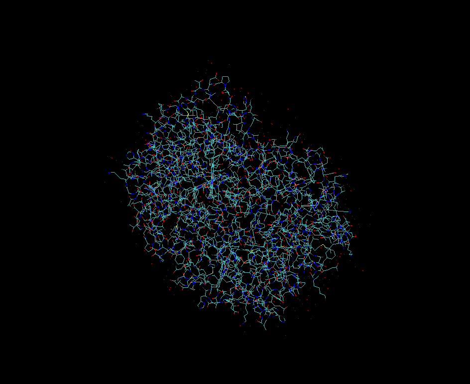
As an example will be using X-ray crystallographic structure of human hemoglobin 1SI4.
Downloading files from Protein Data Bank
VMD can directly query PDB database.
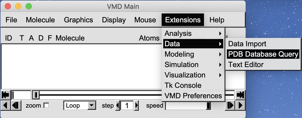
Enter “1si4” and click Load into new molecule in VMD.
Note: loading files from PDB is not possible from compute nodes on all clusters except Cedar because they are not connected to the Internet. Use the login nodes on these systems to download PDB files.
Opening a PDB file saved in your computer.
On a cluster you can download the example PDB file using the following command:
wget https://files.rcsb.org/download/1si4.pdb
If you are using VMD on your local computer you can navigate your browser to the URL above.
Once the file is downloaded, in the VMD Main window menu select File -> New Molecule. The Molecule File Browser window will open. Choose a molecule PDB file.
Understanding information about the loaded molecules
Load a second molecule (you can use the same pdb file), and make sure you have two molecules (ID 0 and 1) loaded.
VMD shows information about loaded molecules in its main window. This window displays:
- molecule ID
- molecule status [T A D F]
- molecule name
- number of atoms
- number of trajectory frames
- volumetric data
- current frame
There are four components to molecular status:
- T (top). Top indicates the default molecule used in the
moltext command. Only one molecule can be top. Some commands such as centering are applied only to the top molecule. - A (active). Several commands such as
Animateoperate on all active molecules. - D (drawn)
- F (fixed)
Fixing molecules
- Fix one of the molecules
- Try using mouse to rotate/translate molecules.
- Delete one of the molecules
Customizing VMD sessions
A few settings often need to be changed from the defaults.
Display rendermode GLSL
The GLSL mode turns on OpenGL extensions implementing programmable shading and transparency for higher quality molecular graphics. This mode renders faster and produces better images than “Normal” mode.- Load 6n4o.pdb file, and create a
NewCartoonrepresentation. Try rotating molecule and observe rendering speed. Is reasonable inNormalmode. - Add
licoricerepresentation. Rendering is very slow now. - Switch to GLSL mode. Performance is better now but still slow. It will improve if more CPUs are available, but the best of course is to use a GPU.
- Load 6n4o.pdb file, and create a
Display Projection orthographic
The orthographic projection allows us to get a better sense of the distance between objects and their relative sizes. The angle of view, distance, and focal length of a camera lens make lines of identical length appear different in perspective mode. Due to this, it is difficult to determine the relative size and dimensions of distant objects in perspective mode.Axes location off
In most cases you don’t want axes to appear in figures prepared for publication.Display depthcue off
The use of depth cues can enhance perception of depth and distance. This is achieved by blending distant objects into the background color. Most of the time, it is not desirable and there are better alternatives.Display ambientocclusion onandMol default material Diffuse
These ray-tracing options enable photorealistic rendering. More about this later.
Interacting with molecules
Obtaining good views for molecules
Rotate, zoom in/out, translate, and set rotation center to get a desired view. Pressing any of these keys switches the mode of interaction. For example, when s key is pressed mouse cursor will change. In this mode click, hold and move on a trackpad/mouse will zoom in/out. If you zoomed too much and don’t see the molecule simply press the = key to reset view.
| Action | Hot keys |
|---|---|
| Rotate | r |
| Zoom (Scale) | s |
| Translate | t |
| Reset View | = |
| Set Center | c |
Working with Graphical Representations
Creating and modifying graphical representations
In the Graphical representations window you can create representations for selected atoms, choose drawing styles and coloring methods
- Ensure 1si4.pdb is loaded
- Navigate to
Graphics–>Representations - Change
Drawing MethodtoNew Cartoon - Change
Coloring MethodtoChain - Try to get a better illumination by moving lights:
Mouse->Move Light
- Try another drawing method:
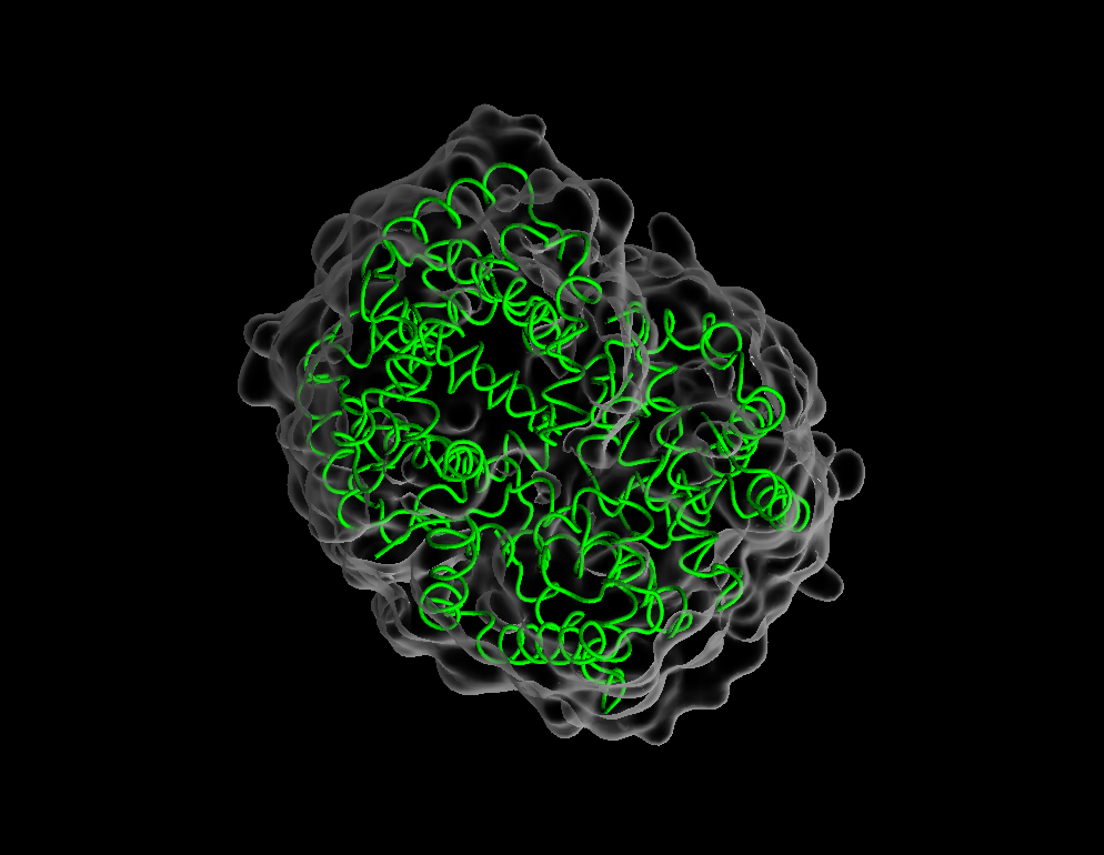
Drawing method–>Tube. - Create a new representation and change its drawing method to
QuickSurf. - Make the surface transparent by changing material to
GlassBubble - Double click to turn representations on/off without deleting them.
- Most useful draw styles:
NewCartoon,QuickSurf,Surf,Licorice,VDW,HBonds
Selecting atoms
In order to make a figure that is clear and impactful, it is useful to display different components of a system using different representations. Selecting groups of atoms is the key to achieving this. Selecting atoms is easy, with lots of options.
- Most often used selection keywords are
noh,backbone,protein,nucleic,resname,resid,index - Selecting a residue:
residue(starts from 0),resid(read from a file) - Selecting an atom:
index(starts from 0),serial(starts from 1) - Use logical operators (and, or, not) for complex selections
- Selecting hetero atoms:
not (protein or nucleic or resname HOH) - Limit selection to one monomer:
chain A - Selecting atoms based on distance:
within 5 of serial 93- selects all atoms located within 3 Angstrom of atom #93same residue as within 5 of serial 93- selects whole residues if any atom is within 5 A of atom #93.
- Selecting groups of atoms or residues
residue 0 to 10, 14, 15, 20 to 30
What selections are available in the loaded molecule?
In the Graphical representations window go to Selections–>Keyword–>chain.
VMD will display all chains in the selected molecule (A,B,C,D). Double click on the Value to select it. To select two or more chains you need to use a command.
Measuring distances, angles, and dihedrals
Use hot keys to measure distances, angles and torsions.
| Action | Hot keys |
|---|---|
| Print info about an atom | 0 |
| Label atom | 1 |
| Measure bond | 2 |
| Measure angle | 3 |
| Measure dihedral | 4 |
How to delete or hide Labels?
Labels can quickly clutter display. How to delete or hide Labels when you don’t need them anymore?
- Deleting labels:
Graphics–>Labels–>Delete
Challenge
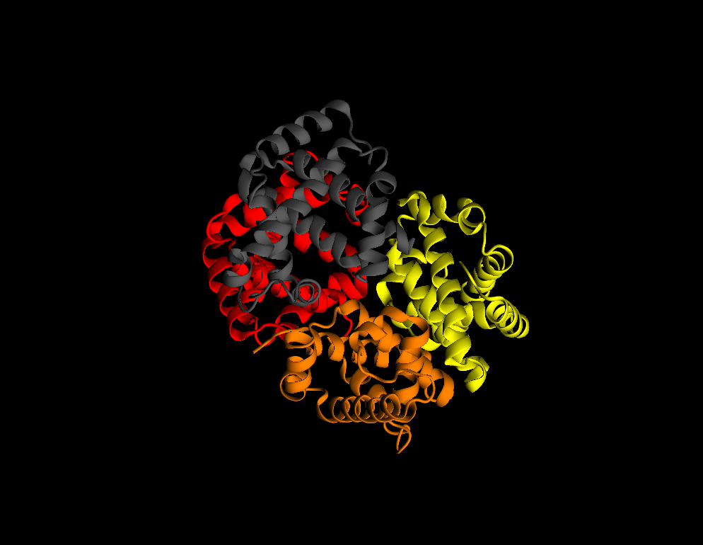
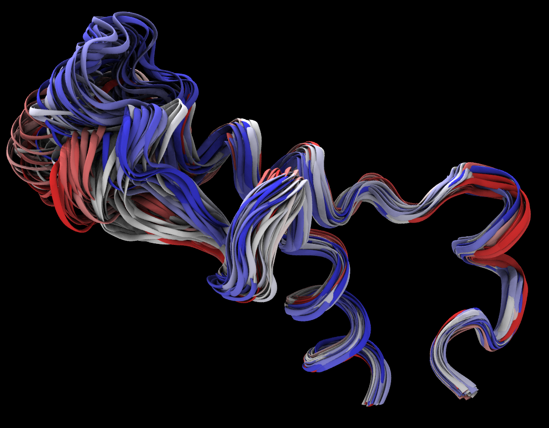
Reproduce the following figure. In this image we see chain A of the pdb entry 1SI4.
The figure shows:
- protein (new cartoon)
- residue HEM (orange licorice)
- HEM atom FE (red CPK)
- HEM ligand residue HIS (yellow licorice)
- HEM ligand residue CYN (yellow VDW).
Use the following selection keywords:
chain,name,resname,same residue as within. You will also need to use logical operatorsand,not.Solution
select chain A
chain Anew cartoon, iceblue, aochalkyselect HEM
chain A and resname HEM
licorice, colorid 3, aochalkySelect atom FE
chain A and name FE
VDW scale 0.4, colorid 1, aochalkySelect only FE ligands
not resname HEM and same residue as within 3 of name FE and chain A
licorice, colorid 4, aochalkyThe previous command selected two FE ligands. How do we select only the small 2-atom FE ligand?
Pick any atom from this molecule. All information about the atom will be printed in the VMD terminal window.select CYN
chain A and resname CYN
surf, colorid 4, aochalky
- save your work:
File->Save visualization state.
Changing default colors
There are 1041 colors available in VMD, with color ids ranging from 0 to 1040. The first 33 are named colors. The remaining group of 1008 are colors used in color maps. There are no names for the specific colors in this group.
Each of the first 33 colors can be modified: Graphics–>Colors–>Color Definitions
Saving your work
- Saving VMD scene:
File->Save visualization state. - Restoring a visualization state:
File->Load visualization state.
A VMD state file is a TCL script that contains all commands used in creating a visualization. You add new commands to a visualization script as you work on it, so it becomes longer and longer. When VMD scripts are executed, they go through all your steps. It is common for intermediary steps to be just trial commands that are not needed to recreate the final version. For example, you created and then deleted some representations, changed colors several times.
In the future, you might want to reuse the visualization scene as a template for visualizing similar molecules. It is a good idea to inspect the visualization state file and keep only the commands necessary to recreate the final scene. In this way, it will remain clear and readable.
Customizing VMD sessions
At startup VMD load a set of default options. You may find that they are not optimal for your work, and you need to change them every time you start a new visualization. Once you have changed settings to your liking you can make them permanent.
Saving current settings
Using the following steps, you can save current settings:
Extensions->VMD Preferences -> Write setting to VMDRC
Managing VMDRC files
VMD preferences are saved in ~/.vmdrc file. VMD creates a very long file containing hundreds of all available settings, even the ones that are using global default values. You may find useful to create a short version of .vmdrc containing only settings that you want to change. A .vmdrc file is just a text file and it can easily be edited manually with any text editor.
Let’s open it. Settings are organized in sections. You don’t want to change default colors, materials or menus. So you can safely delete these sections and leave only display parameters and molecular representations.
As an example, a .vmdrc file might look like this:
      # VMD settings: file ~/.vmdrc

      # Turning-on of menus
      menu main on

      # Change display defaults
      display reposition 100 600
      display resize 672 682
      display projection Orthographic
      display depthcue off
      display rendermode GLSL
      display ambientocclusion on
      axes location Off
      color Display Background white

      # Default material
      mol default material Diffuse

      # Configure keyboard shortcuts
      user add key o {display projection orthographic}
      user add key p {display projection perspective}
Key Points
A first look at the command-line interface
Overview
Teaching: 10 min
Exercises: 5 minQuestions
How to start VMD in text mode?
How to use VMD commands?
Objectives
Learn how to use basic VMD commands
Learn to write loops in VMD
Learn how to get help on VMD commands
Introducing VMD commands
Starting VMD in text mode.
The VMD program can also be used in text mode. Everything you can do in VMD interactively can also be done with commands and scripts. In text mode you interact with VMD using commands. The command-line interface is more flexible than GUI and it allows VMD to read commands from script files. With commands, you can use options than are not available in GUI, and you can run VMD non-interactively. Command-line access to VMD functions is very useful in HPC environment for batch jobs. The text mode is typically used for analyzing MD simulations and rendering animations.
How to start vmd in text mode? If graphical display is not available VMD will automatically fallback into text mode. When you are running analysis scripts on a system with graphical display you may want to enforce text mode to prevent VMD from opening GUI. To do so start vmd with the option -dispdev text.
- The command-line interface
- is more flexible than GUI
- allows VMD to read commands from script files.
- offers options than are not available in GUI
To start vmd in text mode use the option -dispdev text.
Entering commands
Commands can be entered in two ways:
- in the
VMD command window - in
Tk Consoleavailable under theExtensionsmenu
VMD command window is very basic, you can only type commands, and it is not possible to edit command lines. Tk console offers history, autocompletion, and syntax highlighting.
Let’s run our first command.
rotate
rotate usage:
rotate stop -- stop current rotation
rotate [x | y | z] by <angle> -- rotate in one step
rotate [x | y | z] by <angle> <increment> -- smooth transition
If a command is entered without any argument, VMD displays short instructions on how to use it.
rotate x by 90 1
A smooth rotation of the scene around the x axis will be performed with an increment of 1 degree by this command. The advantage of using commands to rotate is that you can precisely specify the angle by which you want to rotate. For example to get a lateral view of a membrane system with membrane in x-y plane you would type rotate x by 90 or rotate y by 90.
Try continuous rotation:
rock x by 1 180
rock off
Sometimes it is useful to set the exact dimensions of the graphical window. For example you want to make a movie in a standard HD format.
Set the exact dimensions of the graphical window.
display resize 1080 720
Sometimes when you start VMD graphical window may be positioned incorrectly so that its menu bar is off screen and you can’t move with mouse. In this case you can reposition it with the command:
Reposition graphical window
display reposition 100 700
- Display position 0 0 corresponds to the lower left display corner.
Get to know more commands
Here are some commands you can run to see how they work:
display resetview
display backgroundgradient on
display projection orthographic
display projection perspective
scale by 2
axes location lowerleft
axes location off
Key Points
Visualizing and analyzing trajectories
Overview
Teaching: 20 min
Exercises: 10 minQuestions
How to load structure files and trajectories into VMD?
How to animate trajectories?
How to generate RMSD data from a trajectory?
Objectives
Learn how to load molecular structure files and MD trajectories.
Learn how to animate trajectories?
Get workshop example data
On the training cluster:
cp /project/60104/workshop_vmd_2024.tar.gz .
tar -xf workshop_vmd_2024.tar.gz
On any other computer:
wget https://github.com/ComputeCanada/molmodsim-amber-md-lesson/releases/download/workshop-2021-04/workshop_vmd_2024.tar.gz
Loading trajectory files
A trajectory file contains the coordinates for all atoms over the course of a simulation. Normally, not every time step of the simulation is saved, since it would create a huge file. It is common to save coordinates every 1000 to 5000 steps. All of these coordinates allow us to measure the dynamic properties of our simulation experiments, including secondary-structure evolution, diffusion constants, correlations between groups, etc
Loading structure files
To load a trajectory, we need both the structure and the trajectory file.
First load a structure file as a new molecule. VMD can read structure files in different formats, such as AMBER7 Parm, XPLOR PSF, GROMACS GRO, PDB, etc.). File types are recognized by extension. If a file has a non-standard extension you can select format manually.
It is best to use structure files that contain connectivity information whenever possible. Examples of file formats with connectivity are molecular topology files or mol2 files. In the absence of connectivity information, VMD uses distances between atoms to determine which ones are connected. Automatic bond determinations does not work perfectly all the time. Stretched bonds may go undetected, and there may be incorrect bonds formed between non-bonded atoms are too close to each other. If you use the wrong bonds, your visualization will be incorrect. The automatic bond determination can be disabled when loading structure files from the command line.
- To load a trajectory, we need both the structure and the trajectory file.
- It is best to use structure files that contain connectivity information whenever possible.
As an example, open Tk Console and run the following commands to load the file 7xcq.pdb without automatic bond determination:
cd ~/workshop_vmd/example_01
mol new 7xcq.pdb autobonds off
Delete all the molecules or restart vmd.
Our training simulation dataset is located in the directory workshop_vmd/example_02. As a structure file we will be using AMBER7 parameter file prmtop_nowat.parm7. Change into this directory and load the topology file.
Once a molecular structure has been loaded you can add a trajectory to it: highlight the molecule, go to File->Load Data into Molecule and choose mdcrd_nowat.xtc. It is a long trajectory with 3000 frames. To make loading faster load every 5th frame.
Loading trajectory using commands on the training cluster
cd ~/workshop_vmd/example_02
mol new prmtop_nowat.parm7
mol addfile mdcrd_nowat.xtc step 5
Viewing AMBER-NetCDF trajectories on Windows and MAC.
NetCDF trajectory files, which are AMBER’s default format, can only be loaded on Linux. You can convert them to GROMACS XTC format by using the CPPTRAJ program from AMBER.
module load ambertools
cpptraj prmtop_nowat.parm7
trajin mdcrd_nowat.nc trajout mdcrd_nowat.xtc go
Visualizing trajectories
- To make trajectory animation run smoother you can interpolate coordinates:
Graphical representations->Trajectory->Trajectory Smoothing Window Size - You can also visualize periodic images:
Graphical representations->Periodic - You can visualize multiple frames and color them by trajectory step. Try resid 809 to 859.
RMSD Trajectory Analysis
The RMSD is a numerical measurement of the difference between two structures: a target structure and a reference structure. Our interest in molecular dynamics is in how structures and parts of structures change over time. For example, a plot of RMSD vs. time will reveal the opening and closing of gates on a protein, such as a transporter. When compared with the starting point, the RMSD can identify protein structure changes and study stability of the simulated system. As the RMSD curve flattens or levels off, that can be a sign that the system has equilibrated.
- You can calculate the time dependence of RMSD in a molecular dynamics simulation using the RMSD Trajectory Tool. It is located under
Extensions->Analysis->RMSD Trajectory Tool
- Load a trajectory
- Start
RMSD Trajectory Tooland add a molecule:Add active Alignall frames using backbone of the whole protein. You can choose a reference frame or a reference molecule.- Make a selection of atoms for which you want to calculate RMSD
- use all protein backbone atoms (normally you don’t want to include hydrogens)
- use all nucleic acid atoms
- use a specific part ot the system (e.g. resid 20 to 80)
- You can optionally save rmsd in a file so you can make a nice figure with your favorite plotting software, and check
Plotbox to view the result.
Calculate the RMSD for two groups of atoms over time
Align frames using backbone of all protein residues. Compute trajectory RMSD for two selections of backbone atoms: residues 790-810 and 820-840.
- Considering both selections, what is the minimum and the maximum RMSD?
- How does the RMSD change when you include all atoms?
- Over the course of the simulation, which of the groups is more stable?
- Are your RMSD results affected by the previous superposition step?
Solution
- The minimum is 0.39, the maximum is 6.1.
- RMSD increases when all atoms are considered.
- The first group, 790-810.
- Yes
RMSD Calculator
The RMSD calculator is similar to the RMSD Trajectory Tool, but it calculates the RMSD between two molecules. It is located under Extensions->Analysis->RMSD Calculator.
Calculation of the RMSD between two molecules
The RMSD calculator works well when two molecules are composed of the same atoms, but the alignment will fail if atom selection in the reference molecule differs from that in the target molecule. The issue is illustrated in this exercise.
- Compute RMSD of two molecules: PDB ID 1si4 and 4n7n. For the calculation, use only chain A backbone atoms.
- When all chain A residues are used for alignment, why does the alignment fail?
- Can you think of a way to include all backbone atoms present in both proteins in the alignment?
If you need to download pdb files use:
wget https://files.rcsb.org/download/4n7n.pdbSolution
- Use the atom selection:
chain A and resid 1 to 140, and check boxBackbone onlyfor both alignment and RMSD calculation, RMSD = 0.92558- The residue 141 of 1si4 molecule has the terminal oxygen atom “OXT”, while it is absent in 4n7n.
- Exclude the OXT atom from the selection:
not name OXT and chain A and resid 1 to 141
Key Points
Visualizing Volumetric Data
Overview
Teaching: 20 min
Exercises: 5 minQuestions
How to visualize volumetric data?
Objectives
Learn how to compute density maps
Learn how to visualize volumes
Visual representations of volumetric data
VMD has the ability to compute and display volumetric data. Volumetric data sets represent parameters whose values depend on their location in 3D, such as density, potential or solvent accessibility. Volumetric datasets store data as 3-D grids. Volumetric data can be visualized by VMD as slices, as isosurfaces, or by using volumetric data to color objects. Plugins for creating and analyzing volumetric data are also available in VMD.
- VMD has the ability to compute and display volumetric data.
Creating density maps
Let’s use the file workshop_vmd/example_03/bcl2-1.pdb
Load this file and compute density map using Volmap Tool:
- Go to
Extensions–>Analysis–>Volmap Tool - Change
selectiontoallandresolutionto0.5 - Press
Create Map
Our molecule now has one volumetric data set associated with it, and isosurface representation of this map is automatically created.
Using slices to visualize volume
- select
VolumeSliceinDrawing Method - select
VolumeinColoring Method - select
Slice angle–>Y
The color scale can be set in Graphics–>Colors–> Color Scale. Select Sequential–>Plasma in Method.
Play with the Slice Offset slider, which adjusts the y-coordinate of the slice. Different colors represent different numerical values of the volumetric data, in this case mass density.
Make slices for the x- and z-directions as well, and rotate you view with the mouse so that all three planes are visible.
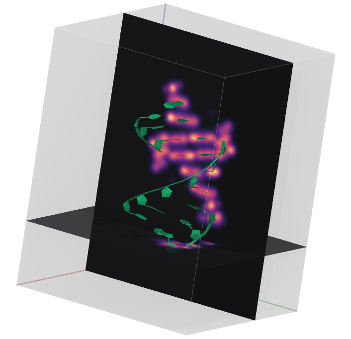
Using isosurfaces to visualize volume
For 3D surface representation of the volumetric data follow the following steps:
- Create a new representation using the
Isosurfacedrawing method. - In the Draw menu, select
Solid Surface.
Now, you can see a surface of constant volumetric value, chosen using the Isovalue slider. As you choose higher values, you see the surface shrinks down around a core where the most average mass was located.
- Select
isovalue 0.1, and change material toGlassBubble. Then create another isosurface withisovalue 2.2and change its color.
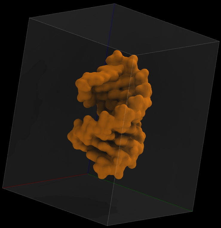
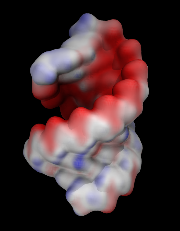
Coloring objects by volumetric data
Another common way to represent volumetric data is by coloring other representations based on it. For example you can color molecular surface by electrostatic potential.
- As an example we will use electrostatic potential saved in the file
workshop_vmd/example_03/bcl2-1_pot.dx
To prepare potential file from the pdb file I first used pdb2pqr web server to prepare pdb file with charges and radii needed for calculation of electrostatic potential. Then I used APBS Electrostatics VMD plugin to compute electrostatic potential around RNA molecule. I will discuss these calculations in detail later. For now we will simply use precomputed potential file as a visualization example.
- Delete the loaded molecule and load bcl2-1.pdb again. Then load data file bcl2-1_pot.dx into the molecule.
- Create
SurforQuickSurfrepresentation. - Color it by volume
- Adjust
Color scale data rangein theTrajectorytab. Try [-50 50].
Visualizing electron density maps
The electron density map represents the fit between the structural model and experimental data from an X-ray structure determination. Scientists commonly use 2fo-fc and fo-fc electron density maps. The fo-fc map shows only the electron density poorly represented by the model, while the 2fo-fc map includes electron density around the model. We will be using the 2fo-fc map for this demonstration.
- Electron density maps calculated using the program DCC can be downloaded in DSN6 format from Structure Summary pages.
Example PDB file is 7xcq.
- Download two files:
The files are available in the folder workshop_vmd/example_04
- Load 7xcq.pdb and then load 7xcq_2fo-fc.dsn6 map into the 7xcq molecule.
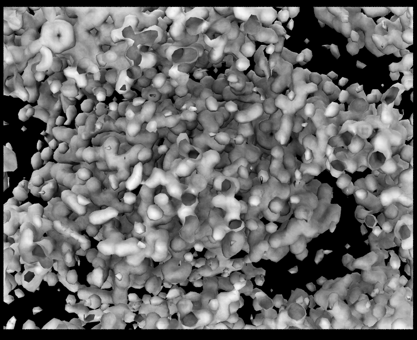
- Create isosurface representation and set the isovalue to 1.0.
The volume map is too big, so the figure is very busy. By focusing on a small area of interest, visualization can be significantly improved. When choosing regions of interest in volumetric data, VMD provides two options.
 Whole Map Whole Map |
 Clipping planes Clipping planes |
 Volime Tool Volime Tool |
Clip Tool
Clipping planes allow for the slicing of a 3D model along a plane. Each molecule can have up to 6 different clipping planes, which can independently be set on or off.
- To get a clear view, use clipping planes to remove volume in front of and behind your region of interest.
Clipping Plane Toolis underExtensions->Visualization. - Check
Normal follows viewbox to orient clipping planes perpendicular to the view direction.
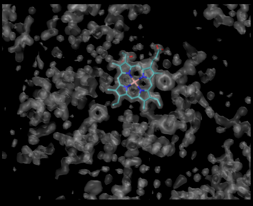
Let’s focus on the HEM. The first step is to orient it in the plane of the screen. Then in the clipping plane tool check the box Normal follows view and activate two clipping planes. Uncheck Normal follows view, rotate the molecule to look at the HEM from its side and adjust positions of the clipping planes.
Volume Tool
- Volume Tool provides many functions for working with volume maps.
- Using the “mask” function you can select a region within a cut-off distance
The “mask” function removes all voxels from an input map that fall outside the given cutoff from a set of atoms. This functionality is available only in VMD command line.
voltool mask <selection> -mol <molID> -vol <volID> -cutoff <cutoff distance>
The voltool operates on selections of atoms, so we need to create a selection.
Let’s select HEM atoms:
atomselect top "resname HEM"
Print all available selections:
atomselect list
You may have more than one selection, so let’s confirm that atomselect0 is the selection we want:
atomselect0 text
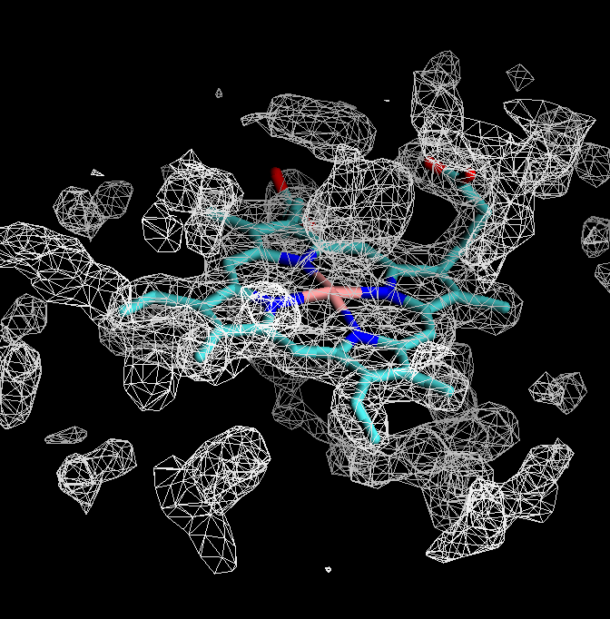
Visualize electron density around HEM:
voltool mask atomselect0 -mol 0 -vol 0 -cutoff 3
Selecting an area of interest with voltool
Visualize electron density around TYR103, or any other residue using voltool.
Key Points
Scripting
Overview
Teaching: 30 min
Exercises: 10 minQuestions
How to work with atom selections?
How to change attributes of selected atoms?
How to move and superimpose selections?
How to write loops
How to measure distances between groups of atoms?
Objectives
Learn to work with atom selections?
Learn to move and superimpose selections?
Learn to write loops in VMD
Learn to measure distances between groups of atoms?
Tcl Scripting in VMD
In addition to commands, VMD offers the built-in Tcl programming language. VMD Tcl scripts can help you investigate molecule properties and perform analysis.
Tcl language
Tcl is shortened form of Tool Command Language. This language combines scripting with an interpreter that gets embedded in the application. There are embedded Tcl interpreters in both VMD and NAMD. Tcl interpreter available from the command-line allows you to write data processing and visualization scripts utilizing any existing VMD functions and variables. For example, you have access to all information about loaded molecules such as coordinates, atom names, occupancy, and charge.
- Tcl interpreter is embedded in both VMD and NAMD.
Selecting atoms
Rotating or translating molecule that we have done so far simply changes viewpoint. It does not change coordinates of the loaded molecules. In your work you may want to rotate or translate a molecule and save its modified coordinates. It may be useful for example if you want to prepare a simulation system containing several copies of a molecule prepared from one structure file.
Many VMD commands operate on selected groups of atoms rather than just on whole molecules. After a selection has been created, it can be modified (rotated, translated), different properties, such as occupancy and beta factors, can be set, and the modified selection can be saved as a file.
- VMD commands operate on selected groups of atoms
As an example, let’s load 1si4.pdb and select protein backbone:
set sel [atomselect top "backbone"]
If command is successful VMD responds with a name of the created selection function:
atomselect0
In your case, the number of the function may be different, depending on how many selections have already been made.
With this command we created a function for selecting atoms, and set a variable sel to point to it. sel is just the name of this variable, you can use any name you wish. You can think of the variable sel as a shortcut to atomselect0. Thus, atomselect0 is equivalent to $sel.
Working with selections
What commands are available for atomselect0?
- To get help on commands available for the function
atomselect0typeatomselect0or$sel.
Try using some of the commands:
$sel num # Returns  the number of atoms
$sel writepdb backbone.pdb # writeXXX where XXX is a known format
$sel writegro backbone.gro
Let’s make another selection using the same variable sel:
set sel [atomselect top "resname CYS and name CA"]
atomselect1
This command resets the variable sel. After this command is executed sel points to atomselect1. This can be verified by displaying the selection text:
$sel text
resname CYS and name CA
What happened to atomselect0?
As you may have thought, atomselect0 as well as any other previously created selections still exist:
atomselect list
Selections can be deleted using the delete command.
atomselect0 delete
Changing properties of selected atoms
We have selected CA atoms of all CYS residues of the protein. Let’s do something useful with this selection:
Find out how may CYS residues are in our protein and what are their ID numbers:
set cys [$sel get resid] # make a list of CYS resid numbers
llength $cys # count the number of elements in the list
We can rename selected atoms:
 $sel set name C1A
 $sel get name
We can manipulate any other attribute of the selection!
Viewing selections
To show a selection in graphical window we first need to choose a drawing method for a new representation and then add the new representation to the molecule:
 mol selection "resname CYS"
 mol representation vdw
 mol addrep top
Moving selected atoms
Translation
$sel moveby {0 50 0}
Complex transformations (rotate + translate)
The move command takes as an argument a [4x4] transformation matrix and applies it to the coordinates of each atom in the selection. A transformation matrix is computed from [3x3] rotation matrix and a translation vector. It is not straightforward to obtain it by hand. VMD has various commands to help creating transformation matrices.
- The
movecommand takes as an argument a [4x4] transformation matrix
The main command for generating transformation matrices is trans. It can create matrices for many transformations such as:
- centering a molecule
- adding an offset
- rotation about any axis {x y z}
- rotation about about a vector
- rotation about a bond
Click here for more details about matrix routines.
Let’s consider examples of some useful transformations.
Rotation around an axis
Rotate a molecule around x-axis by 30 degrees:
set sel [atomselect top all]
$sel move [trans axis x 30]
End of workshop 2024 - 3 hours
Rotation around a bond
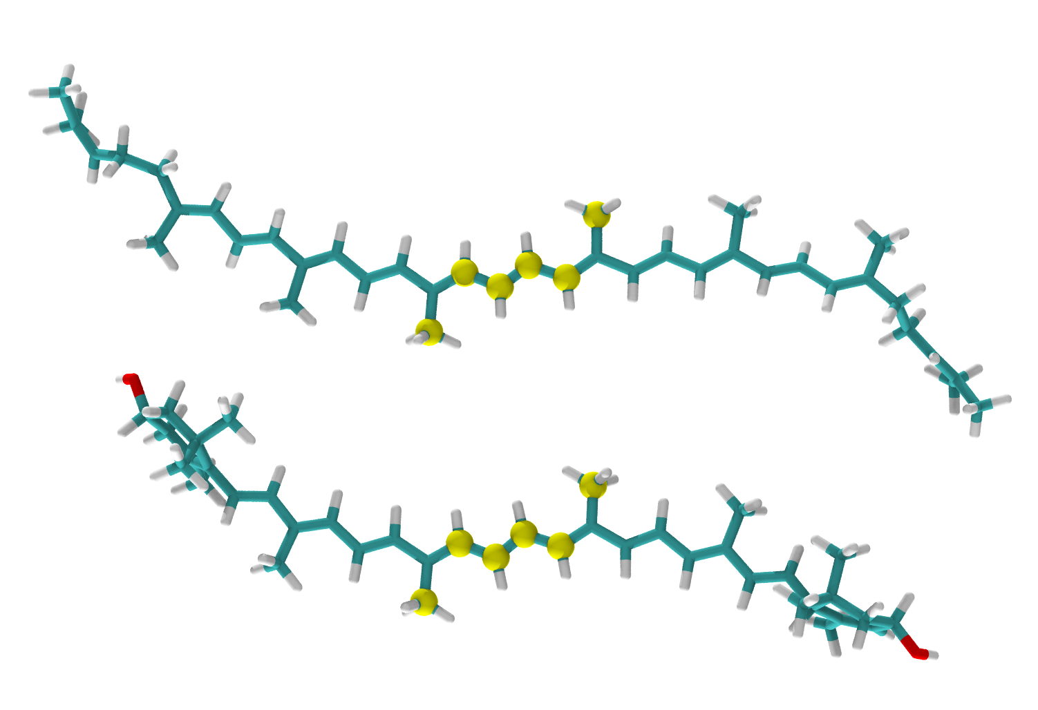
- Convert cis-lutein to trans- by rotating around the bond C15-C35 by 180 degrees.
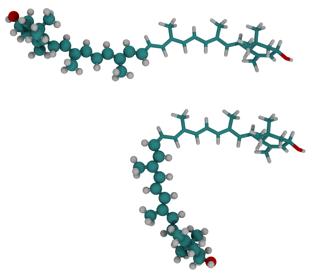
Load the file workshop_vmd/example_05/LUT-noh.pdb
# Select atoms to rotate
set sel [atomselect top "serial 1 to 21"]
# Select rotation axis atoms
set A1 [atomselect top "name C15"]
set A2 [atomselect top "name C35"]
# Get coordinates of these atoms
set AC1 [lindex [$A1 get {x y z}] 0]
set AC2 [lindex [$A2 get {x y z}] 0]
# Rotate selection
$sel move [trans bond $AC1 $AC2 180 deg]
lindex is a builtin Tcl command. It retrieves an element from a list.
Superposing molecules (more challenging)
Although VMD has GUI tool for aligning molecules, it is limited for molecules where lists of equivalent atoms can be constructed using the same selections command. This means that molecules must have either same atom names or same order of atoms. Often this is not the case. For example you may want to align several structurally similar ligands, or two homologous proteins that do not have exactly the same sequence.
With Tcl commands you can construct two independent lists of equivalent atoms and then use them for aligning molecules. The command for generating transformation matrices is measure fit. It creates transformation matrix for aligning two atom selections.
- How to align structurally similar molecules that do not have exactly the same atoms?
As an example, let’s consider two carotenoid molecules: lutein LUT and lycopene LYC.
PDB files of these molecules are in the directory workshop/pdb/carotenoids/.
The following code assumes that ID of the reference molecule is 0 and ID of the molecule that we want to move is 1, so make sure you use the right molecule IDs.
As these molecules have same polyene chains, but different end groups we will use middle part of molecules to align them.
Atoms in these two pdb files are not in the same order, so we need to reorder them.
Selections do not depend on the order in which you list them in the selection command. Selections follow the order in which atoms appear in input files. To solve this problem you need to provide the list describing the order in which the reference atoms should be used to match the fit molecule.
Follow the following steps:
- list atoms in the fit molecule in the order of their index.
- make the list of matching atoms of the reference molecule
- make the list describing the order in which the reference atoms should be used to match the fit molecule
Example:
fitmol C18 C19 C20 C21 C50 C52
refmol C20 C14 C15 C35 C34 C40
order 2 0 1 4 3 5
set fitmol [atomselect 1 "name C18 C19 C20 C21 C50 C52"]
set refmol [atomselect 0 "name C20 C14 C15 C35 C34 C40"]
set trans_mat [measure fit $fitmol $refmol order {2 0 1 4 3 5}]
set allAtoms [atomselect 1 all]
$allAtoms move $trans_mat
Click here for more details
Loops in VMD scripts
Let’s write a simple for loop that animates zooming out.
A loop includes three statement:
- initialization of a loop variable
- termination condition
- increment
There statements are followed by a block of code that is executed repeatedly for each value of the loop variable.
for {set i 0} {$i < 200} {incr i} {scale by 0.99; display update}
Animate cis-trans transition of a lutein molecule
Create a loop that animates lutein’s cis-trans transition. You can use the rotation code that we developed above.
Making input files for NAMD.
NAMD uses beta and occupancy fields of PDB files as an input for various types of calculations. For example, such files are used to define
- position restraint parameters (restraint reference positions and force constant values for each atom)
- temperature coupling parameters (temperature coupling coefficient for each atom).
- constant forces
- collective variables
mol pdbload 1si4
set selAll [atomselect 0 all]
$selAll set occupancy 0
set selBackbone [atomselect 0 "protein and backbone"]
$selBackbone set occupancy 2.0
set selHEM [atomselect 0 "resname HEM"]
$selHEM set occupancy 10.0
$selAll writepdb "constraints.pdb"
Measuring distances between atoms vs. time
Measuring distance between a pair of atoms
Go to the directory with example MD data:
cd ~/scratch/workshop_vmd/example_02
This is a simulation of argonaute protein complexed with microRNA. As an example, let’s measure the distance between some RNA phosphate atoms and sodium ions attached to them.
The following are some pairs you might want to consider:
C895:P, Na+904:Na+
C890:P, Na+1136:Na+
C886:P, Na+1136:Na+
A883:P, Na+966:Na+
mol new prmtop_nowat.parm7
mol addfile mdcrd_nowat.xtc step 5 waitfor all
set file [open "distance.csv" w]
puts $file "Time (ns), Distance (A)"
set nf [molinfo top get numframes]
set sel1 [atomselect top "resid 895 and name P"]
set sel2 [atomselect top "resid 904"]
set bondList [measure bond "[$sel1 get index] [$sel2 get index]" first 0 last $nf]
for {set i 0} {$i < $nf} {incr i} {
   set dist [lindex $bondList $i]
   set time [expr $i/1000.0]
   puts $file "$time, $dist"
   }
close $file
Plotting data with Gnuplot
module load gnuplot
Start Gnuplot by typing gnuplot. Then in gnuplot command prompt enter the following commands:
set xlabel "Time (ns)"
set ylabel "Distance, (A)"
plot "distance.csv"  skip 1 with lines
Measuring distances between groups of atoms
Measure distance between centers of mass of protein and nucleic acids
measure center <selection>- compute coordinates of the center of massvecsub <vec2> <vec1>- find vector connecting two centers of massveclength <vector>- compute distance
mol new prmtop_nowat.parm7
mol addfile mdcrd_nowat.xtc step 5 waitfor all
set file [open "distance.csv" w]
puts $file "Time (ns), Distance (A)"
set nf [molinfo top get numframes]
set prot [atomselect top "noh protein"]
set nucl [atomselect top "noh nucleic"]

for {set i 0} {$i < $nf} {incr i} {
   $prot frame $i
   $nucl frame $i
   set prot_center [measure center $prot weight mass]
   set nucl_center [measure center $nucl weight mass]
   set dist [veclength [vecsub $prot_center $nucl_center]]
   set time [expr $i/1000.0]
   puts $file "$time, $dist"
   }
close $file
Getting help on text commands
You can get help with text commands in several ways:
- This link provides a summary of basic text commands in VMD.
- You can find a detailed description of all commands, as well as their syntax in the online VMD manual.
- Help on commands for atom selections. Type an atom selection function to see a list of commands for it, e.g.
atomselect0. - Builtin Tcl commands: https://www.tcl.tk/man/tcl8.6/TclCmd/contents.html
Useful links: Using the atomselect command
Key Points
Making movies and rendering photorealistic images
Overview
Teaching: 15 min
Exercises: 10 minQuestions
What is Photorealistic Rendering in VMD, and how can I use it?
How to make animations?
Objectives
Learn how to make realistically looking figures
learn to make animations?
How to make 3D objects look more realistic?
VMD is designed to generate images very fast to maximize interactivity, so in rendering in graphical window is optimized for speed. As you may have noticed by now rendered images do not look realistic, they lack 3D feel, they look flat and it is impossible to see surface profile clearly. For example, if you look at the real model of a protein with a cavity you’ll see that the cavity is darker than the exposed outer surface, and becomes darker the deeper inside the cavity one goes.
To simulate such effects one needs to use ray-tracing technique called Ambient Occlusion. The ambient occlusion technique simulates the soft shadows that should naturally occur when indirect or ambient lighting is cast out onto your scene to make 3D objects look more realistic. Another technique helping to simulate a photorealistic image is Depth of Field focal blur.
- The ambient occlusion technique simulates realistic lightning
These features are not enabled by default. Let’s enable ambient occlusion and depth of field focal blur:
Display settings–>Ray-Tracing Optionsand enableAmbient Occlusion,Shading,DoF- You also need to change material to
Diffuseor one of the AO-optimized materials (AoChalky,AoShiny, orAoEdgy). These materials are optimal for rendering with ambient occlusion model. - Finally, use Tachyon a ray-tracing engine that is capable of handling ambient occlusion.
 Snapshot Snapshot |
 Tachyon, AoChalky Tachyon, AoChalky |
 Tachyon, AoEdgy Tachyon, AoEdgy |
Tachyon flavours
VMD provides several implementations of Tachyon:
- Standalone Tachyon, supports rendering with both CPUs and GPUs.
- Internal Tachyon using Intel OSPRay ray-tracing engine (CPU, AVX-accelerated). Best for Intel laptops with integrated graphics.
- Internal Tachyon using NVidia OptiX ray-tracing engine. For computers with NVidia GPUs.
- Interactive Tachyon OptiX allows to setup scene interactively before rendering the final image.
- Tachyon RTX Real Time Ray Tracing. Best for computers with NVidia RTX GPUs (works also on NVidia GPUs without RTX cores).
Tachyon OptiX and Tachyon OSPRay interactive ray tracers
Nvidia OptiX and Intel OSPRay are hardware-accelerated ray tracers capable of interactively rendering photorealistic global illumination. On Alliance systems Tachyon OptiX is available by loading cuda and vmd/1.9.4a43 modules. The interactive ray tracer opens a new graphical window in which you can preview ray-traced rendering and interact with it using a mouse. When you close the interactive window the final image is saved in file. It allows only for a limited interactive functionality. You can rotate, scale, translate with a mouse, and you can turn on/off AO and DoF. It not a full-featured interactive implementation, but it is useful for improving the final rendered image.
Compare normal, glsl and OptiX rendering modes.
Real Time Ray Tracing (RTX-RTRT)
Real Time Ray Tracing solves limitations of the Tachyon OptiX interactive ray tracer by providing full-time ray-tracing in the main OpenGL VMD window.
Real Time Ray Tracing using NVidia RTX cores is supported in version 1.9.4a55 of VMD on Linux platform.
Installation (works on gra-vdi, siku):
# Configure where to install vmd
export VMDHOME=$HOME/scratch/VMD
# There is no need to change anything below this line
export VMDINSTALLBINDIR=$VMDHOME/bin
export VMDINSTALLLIBRARYDIR=$VMDHOME/lib
wget https://www.ks.uiuc.edu/Research/vmd/vmd-1.9.4/files/alpha/vmd-1.9.4a55.bin.LINUXAMD64-CUDA102-OptiX650-OSPRay185-RTXRTRT.opengl.tar.gz
tar -xf vmd-1.9.4a55.bin.LINUXAMD64-CUDA102-OptiX650-OSPRay185-RTXRTRT.opengl.tar.gz
cd vmd-1.9.4a55 && ./configure
cd src && make install
Full-time ray tracing is available as a special rendering mode: rendermode Tachyon RTX RTRT
Pros:
- Enables quick creation of photorealistic animations.
- Greatly simplifies creation of impressive images allowing for an instant feedback.
Cons:
- Not all representations are available.
- Coloring by volume is not available
TachyonLOptiXInternal
- vmd/1.9.4a57 module requires SM80 capable GPU (A100, RTX A5000)
- Downloaded vmd-1.9.4a55 binary works on V100
Tachyon (internal) and standalone
Despite the widespread use of hardware-accelerated Tachyon implementations today, the legacy CPU-only Tachyon implementation is preferred in some cases. Tachyon implementations using OSPay and OptiX libraries can not render representations such as lines, points, and volume slices because they are not available in standard OpenGL libraries.
Tachyon standalone
The standalone version of Tachyon provides greater control over ray-tracing than the internal version. For example:
- You can improve the visual appeal of transparent surfaces by controlling the number of surfaces, for example (shown in Figure below).
- The standalone Tachyon can also be used to render multiple trajectory frames in parallel to accelerate production of high-quality and high-definition animations.
--trans_max_surfaces 1 |
Standalone Tachyon can be installed using the following commands:
export INSTALLDIR=$HOME/bin
mkdir -p $INSTALLDIR
git clone https://github.com/thesketh/Tachyon
cd Tachyon/unix/
make linux-64-thr && ln -s ../compile/linux-64-thr/tachyon $INSTALLDIR
- Check out Publication Figure Rendering With Tachyon for more details.
Making movies
Movie maker
The Movie Maker extension offers several types of animations. You can make a movie of rotation of rocking a static structure, or animate a trajectory with an optional viewpoint rocking. The default compression algorithm is also a very basic quality mpeg-2 encoder optimized for speed on a single computer.
FFmpeg is a powerful tool that can be used to encode videos with high quality codecs. If you haven’t already installed FFmpeg, you can download and install it from here. FFmpeg is already installed on clusters in StdEnv/2023. StdEnv/2020 has it as a module.
Standard options in movie maker are fairly limited. It will simply rotate a molecule or loop over all trajectory frames with a chosen step. If you want to make something more interesting such as zooming at the molecule and moving camera around it then you have to write a script.
Extensions->Visualization->Movie MakerMovie settings->Rotation about Y axisFormat->MPEG2(ffmpeg)- Optionally
Set working directory - In the
Movie durations (seconds)box enter 10 - Press
Make movie
For a trajectory movie duration is defined by the number of frames and trajectory step size. So for 3140 frames with stepsize 2 durarion is 3140/(24fps*2)=65 sec.
Making movies with Tcl scripts (more challenging)
With a custom animation script you have full control of camera movements and special effects such as adding glow lights to some atoms, drawing geometrical figures, slicing volume data, etc.
Much better image rendering can be done in a reasonable time on an HPC cluster. Typically you would use VMD to write scene description files of every trajectory frame for subsequent rendering with a ray tracing engine such as Tachyon. Once input files are ready you submit a script for rendering multiple frames in parallel on hundreds of CPU’s. Then you encode all frames in a video with ffmpeg. Much better compression algorithms such as H.265/HEVC or Google VP9 with much higher quality settings can be used to encode an animation with ffmpeg.
Create a movie showing the diffusion of several Na+ ions.
The animation should look like the one below.
Creating a trajectory movie requires rendering and saving each frame of the trajectory.
- Start with the following script:
mol new prmtop_nowat.parm7
mol addfile mdcrd_nowat.xtc waitfor all

display ambientocclusion on
display shadows on
display aoambient 0.9
display aodirect 0.2
display depthcue off
display projection orthographic
display resize 800 600
#display rendermode {Tachyon RTX RTRT}
axes location off

mol delrep 0 top
# Protein NewCartoon + Licorice
mol selection {protein}
mol representation NewCartoon
mol color ColorID 8
mol material Diffuse
mol addrep top
mol representation Licorice 0.200000 12.000000 12.000000
mol addrep top

# Fix 1: complete the code creating nucleic acids representation
#mol selection ...?
#mol representation ...?
#mol color Charge
#mol material AOShiny
#mol addrep top

# Fix 2: complete the code creating ions representation
#mol selection ...?
#mol representation VDW
#mol color ColorID 22
#mol material ...?
#mol addrep top

# Fix 3: correct the line below to smooth all four representations
foreach i {0 1} { mol smoothrep top $i 5 }

# Fix 4: interactively obtain a good view and set the viewpoint
#molinfo top set {center_matrix rotate_matrix scale_matrix global_matrix} ...?

# Fix 5: change the line below to use all frames, use molinfo to get numframes
set nf 500

for { set i 1; set j 1 } { $i < $nf } { incr i 5; incr j} {
   animate goto $i
   display update
   puts "Rendering frame $i to $j .ppm"
   render snapshot $j.ppm # Graphical display required
   #render TachyonLOptiXInternal $j.ppm  # Nvidia GPU required
}
quit
- Use data in the directory example_02
- You can use selection [resid 966 1136 904 903] for sodium ions. These ions are interesting to show because they display association-dissociation dynamics.
- Viewpoints are defined by four transformation matrices in VMD, and there are methods to get and set them:
 molinfo top get {center_matrix rotate_matrix scale_matrix global_matrix}
 molinfo top set {center_matrix rotate_matrix scale_matrix global_matrix}
- Render frames as *.ppm files using the script:
vmd -e movie_script.vmdCreate a movie from *.ppm files using ffmpeg:
ffmpeg -start_number 1 -i %d.ppm -vcodec libx264 -pix_fmt yuv420p -crf 18 -preset veryslow movie.mp4
- Try adding rotation and scaling:
rotate x by 0.5
scale by 0.995
- Getting rid of translational/rotational motion will improve the animation. Add code aligning each frame to the reference.
Note: with snapshot rendering method display resize in script does not work, set size in ~/.vmdrcSolution
mol new prmtop_nowat.parm7
mol addfile mdcrd_nowat.xtc waitfor all

mol delrep 0 top
mol selection {protein}
mol representation NewCartoon
mol color ColorID 8
mol material Diffuse
mol addrep top
mol representation Licorice 0.200000 12.000000 12.000000
mol addrep top

mol selection {nucleic noh}
mol representation CPK 1.600000 1.400000 12.000000 12.000000
mol color Charge
mol material AOShiny
mol addrep top

mol selection {resid 966 1136 904 903}
mol representation VDW
mol color ColorID 22
mol material AOShiny
mol addrep top

foreach i {0 1 2 3} { mol smoothrep top $i 5 }

display ambientocclusion on
display shadows on
display aoambient 0.9
display aodirect 0.2
display depthcue off
display projection orthographic
display resize 800 600
display rendermode {Tachyon RTX RTRT}
axes location off

# Set viewpoint:
molinfo top set {center_matrix rotate_matrix scale_matrix global_matrix} {{{1 0 0 -60.6021} {0 1 0 -65.806} {0 0 1 -66.7616} {0 0 0 1}} {{0.905554 -0.361229 0.222479 0} {-0.130041 -0.735509 -0.664922 0} {0.403825 0.573183 -0.713014 0} {0 0 0 1}} {{0.0382264 0 0 0} {0 0.0382264 0 0} {0 0 0.0382264 0} {0 0 0 1}} {{1 0 0 -0.02} {0 1 0 -0.08} {0 0 1 0} {0 0 0 1}}}

set ref_sel [atomselect top "protein and backbone" frame 0]
set fit_sel [atomselect top "protein and backbone"]
set all_sel [atomselect top all]

set nf [molinfo top get numframes]
for { set i 1; set j 1 } { $i < $nf } { incr i 5; incr j} {
   $fit_sel frame $i
   $all_sel frame $i
   set trans_mat [measure fit $fit_sel $ref_sel]
   $all_sel move $trans_mat
   animate goto $i
   display update
   puts "Rendering frame $i to $j .ppm"
   render TachyonLOptiXInternal $j.ppm
}
quit
Encoding movies with ffmpeg
- MPEG-2 I-frame only Highest Quality Encoding
ffmpeg -start_number <first_frame> -i %d.ppm -vcodec mpeg2video -pix_fmt yuv420p -q:v 1 -an movie.m2v
- H.264 I-frame only Highest Quality Encoding
ffmpeg -start_number <first_frame> -i %d.ppm -vcodec libx264 -pix_fmt yuv420p -crf 18 -s 1080x720 -preset veryslow movie.mp4
Installing FFMPEG on Windows: Download ffmpeg-git-essentials.7z from https://www.gyan.dev/ffmpeg/builds/
Key Points
Continuum Electrostatics Calculations
Overview
Teaching: 10 min
Exercises: 0 minQuestions
How to compute and visualize electrostatic potential?
Objectives
How to use APBS electrostatics plugin?
Computing electrostatic potential
Surfaces, isosurfaces, and other representations can be colored by electrostatic potential. Any other volumetric properties such as density can be also used for coloring. Electrostatic potential calculations in VMD are done with the Adaptive Poisson-Boltzmann Solver (APBS). APBS solves the equations of continuum electrostatics for biomolecular systems. This means that it computes electrostatic potential for a solvated protein This program must be made available to VMD by loading the apbs module.
To compute electrostatic potential we need a pqr file which is basically pdb file with charges and radii. This file can be made using PDB2PQR web server or utility programs from the ambertools module.
Considering that we will be learning AMBER, let’s use ambertools. There are two steps involved in creating pqr files from pdb files.
Create pdb file with point charges and radii
- Using a force field and a pdb file, create a topology file
module purge
module load StdEnv/2023 ambertools
cd ~/scratch/workshop_vmd/example_03
tleap -f leaprc.RNA.OL3
rna=loadpdb bcl2-1.pdb saveamberparm rna bcl2-1.parm7 bcl2-1.rst7 quit - Use the pdb and the topology file to create the pqr file.
cpptraj bcl2-1.parm7trajin bcl2-1.rst7 trajout bcl2-1.pqr pdb dumpq go quit
Run APBS calculations
Software stack 2020: load apbs and vmd modules
module purge
module load StdEnv/2020 apbs vmd
Software stack 2023: download apbs executable and add path to APBS-3.4.1.Linux/bin
wget https://github.com/Electrostatics/apbs/releases/download/v3.4.1/APBS-3.4.1.Linux.zip
unzip APBS-3.4.1.Linux.zip
setrpaths.sh --path APBS-3.4.1.Linux/bin
Compute electrostatic potential
- Load
bcl2-1.pqr - Create a
QuickSurforSurfrepresentation Extensions->Analysis->APBS electrostatics. UnderEdityou can change calculation settings such as temperature, ion concentration, and dielectric constants. ThenRun APBS- When prompted choose
Load APBS into top molecule - Select coloring method
Volume - Adjust
Color scale data rangein theTrajectorytab. Try [-10 10] - By default potential map
pot.dxis saved in/tmp/apbs.xxxxx. You can change the directory in the top barEdit->Settings.
References
Key Points